This is about coding in R. Please include your R codes and full workings.

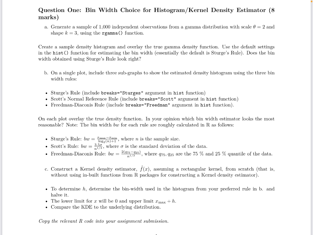
Question One: Bin Width Choice for Histogram/Kernel Density Estimator (8 marks) a. Generate a sample of 1,000 independent observations from a gamma distribution with scale =2 and shape k=3, using the rgamma() function. Create a sample density histogram and overlay the true gamma density function. Use the default settings in the hist () function for estimating the bin width (essentially the default is Sturge's Rule). Does the bin width obtained using Sturge's Rule look right? b. On a single plot, include three sub-graphs to show the estimated density histogram using the three bin width rules: - Sturge's Rule (include breaks="Sturges" argument in hist function) - Scott's Normal Reference Rule (include breaks="Scott" argument in hist function) - Freedman-Diaconis Rule (include breaks= "Freedman" argument in hist function). On each plot overlay the true density function. In your opinion which bin width estimator looks the most reasonable? Note: The bin width bw for each rule are roughly calculated in R as follows: - Sturge's Rule: bw=log2(n)+1xmaxxmin, where n is the sample size. - Scott's Rule: bw=n1/33.5, where is the standard deviation of the data. - Freedman-Diaconis Rule: bw=n1/32(q75q25), where q75,q25 are the 75% and 25% quantile of the data. c. Construct a Kernel density estimator, f^(x), assuming a rectangular kernel, from scratch (that is, without using in-built functions from R packages for constructing a Kernel density estimator). - To determine h, determine the bin-width used in the histogram from your preferred rule in b. and halve it. - The lower limit for x will be 0 and upper limit xmax+h. - Compare the KDE to the underlying distribution. Copy the relevant R code into your assignment submission. Question One: Bin Width Choice for Histogram/Kernel Density Estimator (8 marks) a. Generate a sample of 1,000 independent observations from a gamma distribution with scale =2 and shape k=3, using the rgamma() function. Create a sample density histogram and overlay the true gamma density function. Use the default settings in the hist () function for estimating the bin width (essentially the default is Sturge's Rule). Does the bin width obtained using Sturge's Rule look right? b. On a single plot, include three sub-graphs to show the estimated density histogram using the three bin width rules: - Sturge's Rule (include breaks="Sturges" argument in hist function) - Scott's Normal Reference Rule (include breaks="Scott" argument in hist function) - Freedman-Diaconis Rule (include breaks= "Freedman" argument in hist function). On each plot overlay the true density function. In your opinion which bin width estimator looks the most reasonable? Note: The bin width bw for each rule are roughly calculated in R as follows: - Sturge's Rule: bw=log2(n)+1xmaxxmin, where n is the sample size. - Scott's Rule: bw=n1/33.5, where is the standard deviation of the data. - Freedman-Diaconis Rule: bw=n1/32(q75q25), where q75,q25 are the 75% and 25% quantile of the data. c. Construct a Kernel density estimator, f^(x), assuming a rectangular kernel, from scratch (that is, without using in-built functions from R packages for constructing a Kernel density estimator). - To determine h, determine the bin-width used in the histogram from your preferred rule in b. and halve it. - The lower limit for x will be 0 and upper limit xmax+h. - Compare the KDE to the underlying distribution. Copy the relevant R code into your assignment submission