this is all one question!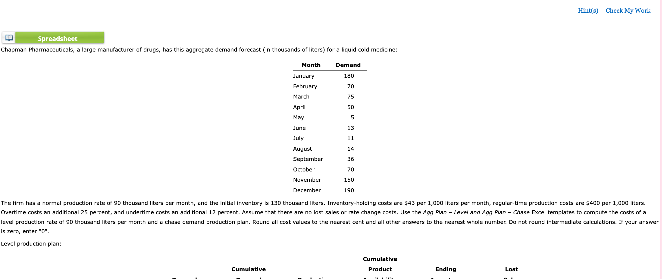

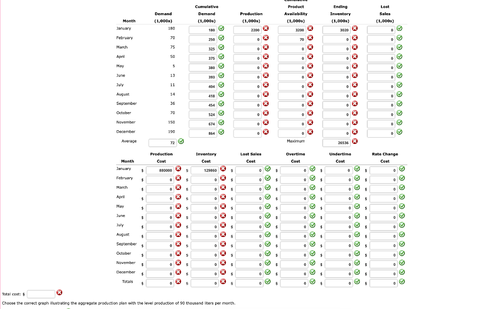
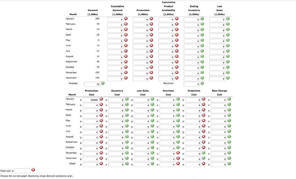
Hint(s) Check My Work Spreadsheet Chapman Pharmaceuticals, a large manufacturer of drugs, has this aggregate demand forecast (in thousands of liters) for a liquid cold medicine: Month Demand 180 January February March 70 75 50 April May June 5 13 July 11 14 August September 36 October 70 November 150 December 190 The firm has a normal production rate of 90 thousand liters per month, and the initial inventory is 130 thousand liters. Inventory-holding costs are $43 per 1,000 liters per month, regular-time production costs are $400 per 1,000 liters. Overtime costs an additional 25 percent, and undertime costs an additional 12 percent. Assume that there are no lost sales or rate change costs. Use the Agg Plan - Level and Agg Plan - Chase Excel templates to compute the costs of a level production rate of 90 thousand liters per month and a chase demand production plan. Round all cost values to the nearest cent and all other answers to the nearest whole number. Do not round intermediate calculations. If your answer is zero, enter "O". Level production plan: Cumulative Cumulative Product Ending Lost Cumulative Demand (1,000) Demand (1,000) 160 Product Availability (1,000) 32003 Ending Inventory (1,000) Lost Sales (1,000) Month January Production (1,000) X 2200 o 180 3020 0 February 70 70 X 0 0 250 325 March 75 o 0 0 o 0 o 3 April 50 375 0 og May 5 0 0 0 June 03 0 o 3 380 393 404 13 0 0 o 0 o o 3 July 11 0 o 0 14 * 418 0 0 0 August September 0 og 36 454 0 0 o o 3 X October 70 0 0 524 674 November 150 0 0 X 0 03 0 % O 26536 December 190 864 0 x og Average 72 Maximum Production Lost Sales Undertime Inventory Cost Overtime Cost Rate Change Cost Cost Cost Cost Month January $ 880000 s $ 129860s 0 0 $ 0 o o 0 February $ 0 0 s 0 $ 0 $ 0 March $ 0 $ D $ 0 $ 0 $ 0 $ 0 April $ $ D $ 0 $ o + 0 May o $ X 0 $ $ 0 $ 0 $ 0 $ o June $ 0 $ 0 0 0 0 July $ 0 X $ D $ 0 $ 0 $ 0 $ 0 August $ 0 $ D S $ 0 $ o $ $ September $ 0 X $ 03 D $ 0 0 $ 0 $ og og og og October $ 0 $ 0 $ 0 o $ 0 $ November $ 0 X $ $ 0 $ 0 $ 0 $ 0 $ December $ $ 0 X $ 0 $ 0 $ o 0 $ 0 $ 0 Totals $ 0 $ D X S 0 $ 0 $ 0 $ og Total cost: Choose the correct graph illustrating the aggregate production plan with the level production of 90 thousand liters per month Cumulative Product Availability (1,000) Cumulative Demand (1,000) Demand (1,000) 180 Ending Inventory (1,000) Production (1,000) 3 Month January Lost Sales (1,000) 0 0 0 0 February 70 0 0 o 0 0 og D March 75 0 0 April SO 0 0 . o o 0 0 May 5 0 0 0 D June 13 o 0 0 July 11 0 0 0 0 o o 3 o o August 14 0 0 3 0 D September 35 03 0 0 October 70 0 0 0 og 0 November 150 0 o 0 December 190 0 0 Average 72 Maximum 0 Production Lost Sales Rate Change Inventory Cost Overtime Cost Undertime Cost Month Cost Cost Cost January $ 154000 s s o X $ 0 S 0 $ 0 s 0 February $ 0 S 0 $ 0 S 0 $ 0 0 March $ 0 s 0 $ 0 s 0 $ 03 s 0 April $ 0 X s 0 $ 0 S 0 $ 0 o S 0 May $ 0 S 0 0 S 0 $ 0 S o June $ 0 s 0 $ 0 s 0 $ 0 s 0 July $ 0 s 0 0 s 5 o $ 0 s s 0 0 S 0 $ 0 S 0 $ August $ September $ 0 o 0 0 s S 0 $ 0 s 0 $ s 0 October $ 0 s 0 0 5 0 $ 0 s 0 November * $ 0 0 S 0 S 0 . o 3 0 $ $ 0 0 $ $ December $ 0 s 0 $ 0 S 0 s 0 Tatals 0 $ s 0 ex $ 0 s 0 og 0 $ s 0 3 Total cost: $ Choose the correct graph illustrating chase demand production plan