this is an excel project

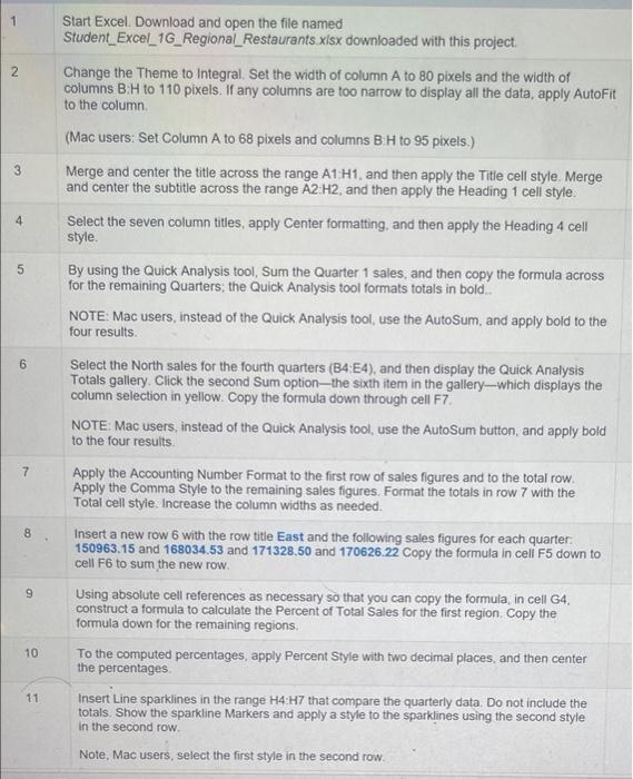
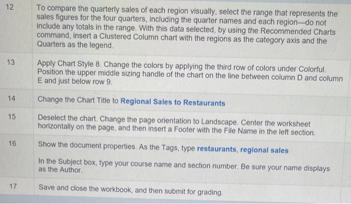
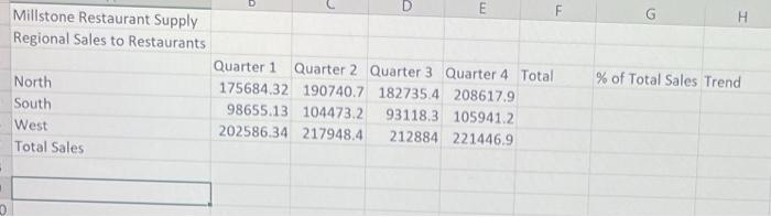
2 3 4 5 03 6 Start Excel. Download and open the file named Student_Excel_1G_Regional_Restaurants.xlsx downloaded with this project, Change the Theme to Integral. Set the width of column A to 80 pixels and the width of columns BiH to 110 pixels. If any columns are too narrow to display all the data, apply AutoFit to the column (Mac users: Set Column A to 68 pixels and columns BiH to 95 pixels.) Merge and center the title across the range A1:H1, and then apply the Title cell style. Merge and center the subtitle across the range A2:H2, and then apply the Heading 1 cell style. Select the seven column titles, apply Center formatting, and then apply the Heading 4 cell style By using the Quick Analysis tool, Sum the Quarter 1 sales, and then copy the formula across for the remaining Quarters, the Quick Analysis tool formats totals in bold NOTE: Mac users, instead of the Quick Analysis tool, use the AutoSum, and apply bold to the four results. Select the North sales for the fourth quarters (B4:E4), and then display the Quick Analysis Totals gallery. Click the second Sum optionthe sixth item in the gallery--which displays the column selection in yellow. Copy the formula down through cell F7 NOTE Mac users, instead of the Quick Analysis tool, use the AutoSum button and apply bold to the four results Apply the Accounting Number Format to the first row of sales figures and to the total row. Apply the Comma Style to the remaining sales figures. Format the totals in row 7 with the Total cell style. Increase the column widths as needed. Insert a new row 6 with the row title East and the following sales figures for each quarter. 150963.15 and 168034.53 and 171328.50 and 170626.22 Copy the formula in cell F5 down to cell F6 to sum the new row. Using absolute cell references as necessary so that you can copy the formula, in cell G4 construct a formula to calculate the Percent of Total Sales for the first region. Copy the formula down for the remaining regions To the computed percentages, apply Percent Style with two decimal places, and then center the percentages Insert Line sparklines in the range H4 H7 that compare the quarterly data. Do not include the totals. Show the sparkline Markers and apply a style to the sparklines using the second style 7 8 9 10 11 in the second row Note, Mac users, select the first style in the second row. 12 To compare the quarterly sales of each region visually, select the range that represents the sales figures for the four quarters, including the quarter names and each region-do not include any totals in the range. With this data selected, by using the Recommended Charts command, insert a Clustered Column chart with the regions as the category axis and the Quarters as the legend. 13 Apply Chart Style 8. Change the colors by applying the third row of colors under Colorful. Position the upper middle sizing handle of the chart on the line between column D and column E and just below row 9. 14 Change the Chart Title to Regional Sales to Restaurants 15 Deselect the chart. Change the page orientation to Landscape. Center the worksheet horizontally on the page, and then insert a Footer with the File Name in the left section 16 Show the document properties. As the Tags, type restaurants, regional sales In the Subject box, type your course name and section number. Be sure your name displays as the Author 17 Save and close the workbook, and then submit for grading. G H D E F Millstone Restaurant Supply Regional Sales to Restaurants Quarter 1 Quarter 2 Quarter 3 Quarter 4 Total North 175684.32 190740.7 182735.4 208617.9 South 98655.13 104473.2 93118.3 1059412 West 202586.34 217948.4 212884 221446.9 Total Sales % of Total Sales Trend