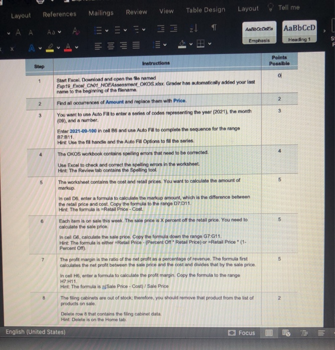
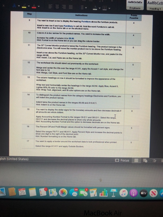
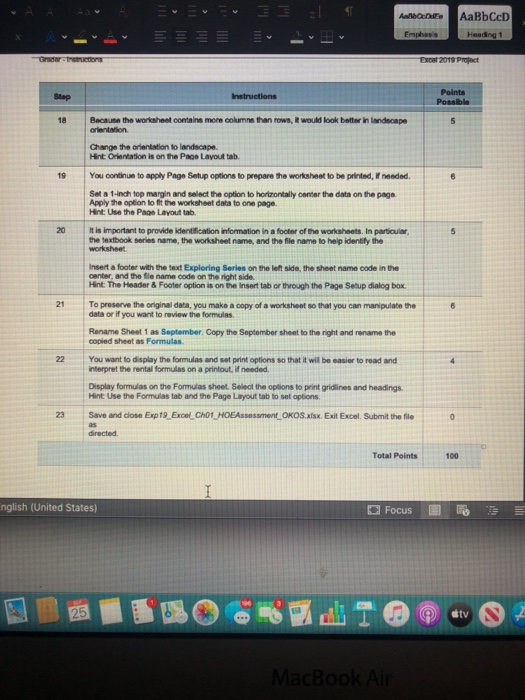
View Layout Tell me Mailings Review Table Design Layout References A A zt ANADO DE AaBbCcD Emphasis Heading 1 Instructions Points Possible Step 1 2 2 3 4 5 5 Start Excel. Download and open the file named Exp19 Excel Ch01 HOE Assessment_OKOS.xlsx Grader has automatically added your last name to the beginning of the filename Find all occurrences of Amount and replace them with Price. 3 You want to use Auto Fil to enter a series of codes representing the year (2021), the month (09), and a number. Enter 2021-09-100 in coll 86 and use Auto Fil to complete the sequence for the range B7B11 Hint Use the fil handle and the Auto Fill Options to fill the series. The OKOS workbook contains spelling errors that need to be corrected. Use Excel to check and correct the spelling errors in the worksheet. Hint: The Review tab contains the Spelling tool. The worksheet contains the cost and retail prices. You want to calculate the amount of markup In cell D6, enter a formula to calculate the markup amount, which is the difference between the retail price and cost. Copy the formula to the range 07:011 Hint: The formula is Retail Price - Cost. Each item is on sale this week. The sale price is X percent off the retail price. You need to calculate the sale price In cell G6, calculate the sale price. Copy the formula down the range G7:611. Hint: The formula is either =Retail Price - (Percent of Retail Price) or Retail Price' (1- Percent off). The profit margin is the ratio of the net profit as a percentage of revenue. The formula first calculates the net profit between the sale price and the cost and divides that by the sale price In cell H6, enter a formula to calculate the profit margin. Copy the formula to the range H7 H11 Hint: The formula is a/Sale Price - Cost) / Sale Price The filing cabinets are out of stock; therefore, you should remove that product from the list of products on sale Delete row 8 that contains the filing cabinet data. Hint: Delete is on the Home tab, English (United States) Focus 5 6 7 5 2 2 AWD AaBbCcD Heading 1 Emphasis Step Possible 4 You want to set a row to the heating Furniture above ramuroducts Instanewrow and type Furniture in A Bold the word umre AR Mais on the Home on the three 10 11 8 Com A is loow for the products. You want to increase the width Increase the width of column A to 20.00 Hint Format is on the Hansetab or you can drag the con bonde The 37" Curved to product is below the Future heading. This product belongs in the Bere you will move the monitor product row to be above the Future heading ar now above the Future heading out the 37" Curved Monitorow, and paste in the range AB.H. Mint Insert, Cut, and Pastewe on the Home tab The worksheet te should stand out prominently on the worksheet Merge and enter the over the range A1.ht, apply the Accent 1 col style and change the forts to 14 Hint: Marge, Call Style, and Font Size on the Home tab The column headings on row & should be formatted to improve the appearance of the 12 5 13 6 14 5 15 Wrap test and horny center the headings in the web Apply Accent Light 80% color to the range Hint Wrap Text, alignment and color options are on the Home tab. To distinguish the product names from the category Madinga Dectronics and Pumture, you wil indent the product names Inden wice the product names in the range A6 Aland A10 A11 Hint Indent is on the Home You want to display the dollar signs for the monetary amounts and then decrease decimal all amounts are whole dos Apply Accounting Number Format to the gas CET1 and 4911. Select one CHC11 and decrease the decimal places to show only whole ounts Hint Accounting Number Format and the option to decrease dels are on the Home tab The Percent off and Profit Margin values should be formatted with percent signs Select the ranges F&F11 and 16H11 Apply Percent style and worse the decimal points to show one digit is the right of the decimal point Hint Number formatting is on the Home tab, You want to apply a border around the worksheet data to look professional when we Select the range A1 Handply Outside Borders 16 5 17 glish (United States) Focus 25 tv MacBook Air ADE Il lali AaBbCcD Heading 1 Emphasis Gertruction Excel 2019 Project Stap Instructions Points Possible 18 5 19 6 20 Because the worksheet contains more columns than rows, it would look botter in landscape orientation Change the orientation to landscape Hint Orientation is on the Page Layout tab. You continue to apply Pago Setup options to prepare the worksheet to be printed, I needed. Set a 1-inch top margin and select the option to horizontally center the data on the page. Apply the option to fit the worksheet data to one page. Hint: Use the Page Layout tab. It is important to provide identification Information in a footer of the worksheets. In particular, the textbook series name, the worksheet name, and the file name to help identify the worksheet Insert a footer with the text Exploring Series on the left side, the sheet name code in the Hint The Header & Footer option is on the Insert tab or through the Page Setup dialog box. To preserve the originaldate, you make a copy of a worksheet so that you can manipulate the data or if you want to review the formulas. Rename Sheet 1 as September. Copy the September sheet to the right and rename the copied sheet as Formulas. You want to display the formulas and set print options so that it will be easier to read and interpret the rental formulas on a printout needed Display formulas on the Formulas sheet. Select the options to print gridlines and headings Hint Use the Formulas tab and the Page Layout tab to sat options Save and close Exp19_Excwl_CHOT HOEA estOKOS.xlsx. Exit Excel. Submit the file directed 21 6 22 23 0 Total Points 100 English (United States) Focus 25 tv MacBook Air View Layout Tell me Mailings Review Table Design Layout References A A zt ANADO DE AaBbCcD Emphasis Heading 1 Instructions Points Possible Step 1 2 2 3 4 5 5 Start Excel. Download and open the file named Exp19 Excel Ch01 HOE Assessment_OKOS.xlsx Grader has automatically added your last name to the beginning of the filename Find all occurrences of Amount and replace them with Price. 3 You want to use Auto Fil to enter a series of codes representing the year (2021), the month (09), and a number. Enter 2021-09-100 in coll 86 and use Auto Fil to complete the sequence for the range B7B11 Hint Use the fil handle and the Auto Fill Options to fill the series. The OKOS workbook contains spelling errors that need to be corrected. Use Excel to check and correct the spelling errors in the worksheet. Hint: The Review tab contains the Spelling tool. The worksheet contains the cost and retail prices. You want to calculate the amount of markup In cell D6, enter a formula to calculate the markup amount, which is the difference between the retail price and cost. Copy the formula to the range 07:011 Hint: The formula is Retail Price - Cost. Each item is on sale this week. The sale price is X percent off the retail price. You need to calculate the sale price In cell G6, calculate the sale price. Copy the formula down the range G7:611. Hint: The formula is either =Retail Price - (Percent of Retail Price) or Retail Price' (1- Percent off). The profit margin is the ratio of the net profit as a percentage of revenue. The formula first calculates the net profit between the sale price and the cost and divides that by the sale price In cell H6, enter a formula to calculate the profit margin. Copy the formula to the range H7 H11 Hint: The formula is a/Sale Price - Cost) / Sale Price The filing cabinets are out of stock; therefore, you should remove that product from the list of products on sale Delete row 8 that contains the filing cabinet data. Hint: Delete is on the Home tab, English (United States) Focus 5 6 7 5 2 2 AWD AaBbCcD Heading 1 Emphasis Step Possible 4 You want to set a row to the heating Furniture above ramuroducts Instanewrow and type Furniture in A Bold the word umre AR Mais on the Home on the three 10 11 8 Com A is loow for the products. You want to increase the width Increase the width of column A to 20.00 Hint Format is on the Hansetab or you can drag the con bonde The 37" Curved to product is below the Future heading. This product belongs in the Bere you will move the monitor product row to be above the Future heading ar now above the Future heading out the 37" Curved Monitorow, and paste in the range AB.H. Mint Insert, Cut, and Pastewe on the Home tab The worksheet te should stand out prominently on the worksheet Merge and enter the over the range A1.ht, apply the Accent 1 col style and change the forts to 14 Hint: Marge, Call Style, and Font Size on the Home tab The column headings on row & should be formatted to improve the appearance of the 12 5 13 6 14 5 15 Wrap test and horny center the headings in the web Apply Accent Light 80% color to the range Hint Wrap Text, alignment and color options are on the Home tab. To distinguish the product names from the category Madinga Dectronics and Pumture, you wil indent the product names Inden wice the product names in the range A6 Aland A10 A11 Hint Indent is on the Home You want to display the dollar signs for the monetary amounts and then decrease decimal all amounts are whole dos Apply Accounting Number Format to the gas CET1 and 4911. Select one CHC11 and decrease the decimal places to show only whole ounts Hint Accounting Number Format and the option to decrease dels are on the Home tab The Percent off and Profit Margin values should be formatted with percent signs Select the ranges F&F11 and 16H11 Apply Percent style and worse the decimal points to show one digit is the right of the decimal point Hint Number formatting is on the Home tab, You want to apply a border around the worksheet data to look professional when we Select the range A1 Handply Outside Borders 16 5 17 glish (United States) Focus 25 tv MacBook Air ADE Il lali AaBbCcD Heading 1 Emphasis Gertruction Excel 2019 Project Stap Instructions Points Possible 18 5 19 6 20 Because the worksheet contains more columns than rows, it would look botter in landscape orientation Change the orientation to landscape Hint Orientation is on the Page Layout tab. You continue to apply Pago Setup options to prepare the worksheet to be printed, I needed. Set a 1-inch top margin and select the option to horizontally center the data on the page. Apply the option to fit the worksheet data to one page. Hint: Use the Page Layout tab. It is important to provide identification Information in a footer of the worksheets. In particular, the textbook series name, the worksheet name, and the file name to help identify the worksheet Insert a footer with the text Exploring Series on the left side, the sheet name code in the Hint The Header & Footer option is on the Insert tab or through the Page Setup dialog box. To preserve the originaldate, you make a copy of a worksheet so that you can manipulate the data or if you want to review the formulas. Rename Sheet 1 as September. Copy the September sheet to the right and rename the copied sheet as Formulas. You want to display the formulas and set print options so that it will be easier to read and interpret the rental formulas on a printout needed Display formulas on the Formulas sheet. Select the options to print gridlines and headings Hint Use the Formulas tab and the Page Layout tab to sat options Save and close Exp19_Excwl_CHOT HOEA estOKOS.xlsx. Exit Excel. Submit the file directed 21 6 22 23 0 Total Points 100 English (United States) Focus 25 tv MacBook Air