This is PolynomialDemo

%% LINEAR ALGEBRA DEMONSTRATION % __ __ ______ ____ % /\ \/\ \/\__ _\/\ _`\ % \ \ \ \ \/_/\ \/\ \ \/\ \ % \ \ \ \ \ \ \ \ \ \ \ \ \ % \ \ \_\ \ \ \ \ \ \ \_\ \ % \ \_____\ \ \_\ \ \____/ % \/_____/ \/_/ \/___/ % Instructor: Dr. Chin-Tuan Tan % TA: Mehrdad Heydarzadeh % The University of Texas at Dallas % Spring 2017 % % This code is a demonstration for least square concept and its % applications. %% DATA SET % The dataset in this demonstration is provided by Earth science % communication team at NASA JPL, Caltech which is publicly available for % download via https://climate.nasa.gov/vital-signs/global-temperature % The time series below shows the five-year average variation of global % surface temperatures from 1884 to 2016. % Each sample in data shows the difference of temperature to previous year. % In our Demo the time series is stored in a mat file called Data.mat and % it has variables Time and Temp.

%Load the data clf; load ('Testdata.mat'); %plot Data h=figure(); plot(x,y,'bo'); xlabel ('x'); ylabel('y'); %% Problem Definition % The data is available from 1984 to 2016. But we assume that we are in % 2013 and we do not have access to data from 2014-2016. Our goal is to % build a model for making prediction for these three years. Then we can % verify the accuracy of our method by read data from these three years. % So, we devide the dataset into two parts. Train for builing model % (1984-2013) and test for verifying the accuracy (2013-2016). Also, for % mathematical simplicity we subtract Time variable by 1984 to have small % numbers. So, 1984 is mapped to 0 and 1985 is mapped to 1 and so on.

t=x - 1984; % Change of variable for time. %Traing set tTrain = t(1:end-3); xTrain = y(1:end-3); %Test set tTest = t(end-2:end); xTest= y(end-2:end); %plot again clf; hold on; plot(tTrain,xTrain,'bo'); plot(tTest,xTest,'ro'); xlabel ('x'); ylabel('y'); legend( 'Train data','Test data','location','NW');

%% Linear Model % The first model that we are going to test is the linear model. Although % by looking at the plot it is clear that linear assumption is not a very % valid assumption, it is the simples model that we can imagine.

% All over this demo we have a system like Ax=b where b is the temperature, % x is the vector of unknowns in the model (for exaple for a linear model % like y=at+b, x is [ b a]'). and A is the matrix of regressors. This % matrix % is a function of input variable (t) and the model structure.

l = numel(tTrain); % Number of samples in training set b=xTrain; A=[ones(l,1) tTrain]; % The solution for regression is x= inverse(A'A)*A'b xl=pinv(A'*A)*(A')*b; %plot the models out xhat = xl(1) + xl(2)*t; plot(t,xhat);

%% Quadratic Model % As you can seen the prediction of linear model is so poor. It can't even % get the trend in training data. So, we increase the complexity of model % by choosing a quadratic model. For this purpose, we need to modify the % matrix A.

A=[ones(l,1) tTrain tTrain.^2]; xq=pinv(A'*A)*(A')*b; xhat = xq(1) + xq(2)*t + xq(3)*t.^2; plot(t,xhat);

%% Cubic Model % Quadratic model has a better accuracy in comparison to linear but it is % not enough yet. So, we increase the order of model

A=[ones(l,1) tTrain tTrain.^2 tTrain.^3]; xc=pinv(A'*A)*(A')*b; xhat = xc(1) + xc(2)*t + xc(3)*t.^2 + xc(4)*t.^3; plot(t,xhat);

%% Higher order Models % Quadratic model has a better accuracy in comparison to linear but it is % not enough yet. So, we increase the order of model

A=[ones(l,1) tTrain tTrain.^2 tTrain.^3 tTrain.^4]; xh=pinv(A'*A)*(A')*b; xhat = xh(1) + xh(2)*t + xh(3)*t.^2 + xh(4)*t.^3 + xh(5)*t.^4; plot(t,xhat);

%% Measuring the prediction error % In this section we measure the estimation error of each model %linear xTestHat = xl(1)+xl(2)*tTest; el = sum((xTest-xTestHat).^2); %Quadratic xTestHat = xq(1)+xq(2)*tTest+xq(3)*tTest.^2; eq = sum((xTest-xTestHat).^2); %Cubic xTestHat = xc(1)+xc(2)*tTest+xc(3)*tTest.^2 +xc(4)*tTest.^3; ec = sum((xTest-xTestHat).^2); %High Order Model (4th order) xTestHat = xh(1)+xh(2)*tTest+xh(3)*tTest.^2+xh(4)*tTest.^3+xh(5)*tTest.^4; eh = sum((xTest-xTestHat).^2);

display(el); display(eq); display(ec); display(eh);

In Part I of the project in " PolynomialDemo " file, the input variable is Time and the output is Temp. However, in the Part II, in the attached mat file, the input variable is x and the output variable is y. So, if you are considering resuing the PolynomialDemo code, you need to consider this name difference.

How do I do this using matlab?

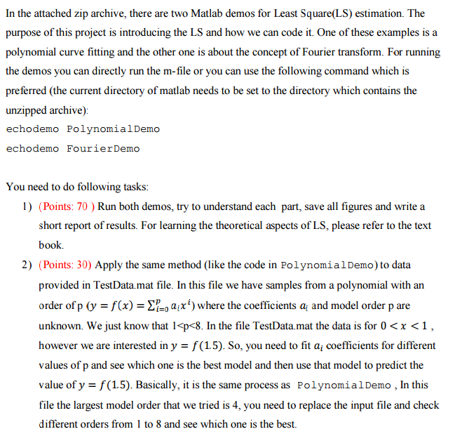
In the attached zip archive, there are two Matlab demos for Least Square(LS) estimation. The purpose of this project is introducing the LS and how we can code it. One of these examples is a polynomial curve fitting and the other one is about the concept of Fourier transform. For running the demos you can directly run the m-file or you can use the following command which is preferred (the current directory of matlab needs to be set to the directory which contains the unzipped archive) echodemo Polynomial Demo echodemo Fourier Demo You need to do following tasks l) (Points: 70 Run both demos, try to understand each part, save all figures and write a short report of results. For learning the theoretical aspects of LS, please refer to the text book. 2) (Points: 30) Apply the same method (like the code in PolynomialDemo) to data provided in TestData.mat file. In this file we have samples from a polynomial with an order of p f(x): auxi) where the coefficients ai and model order p are unknown. We just know that 1