this is wolfram mathematica. i already did the first half, need help on other half.

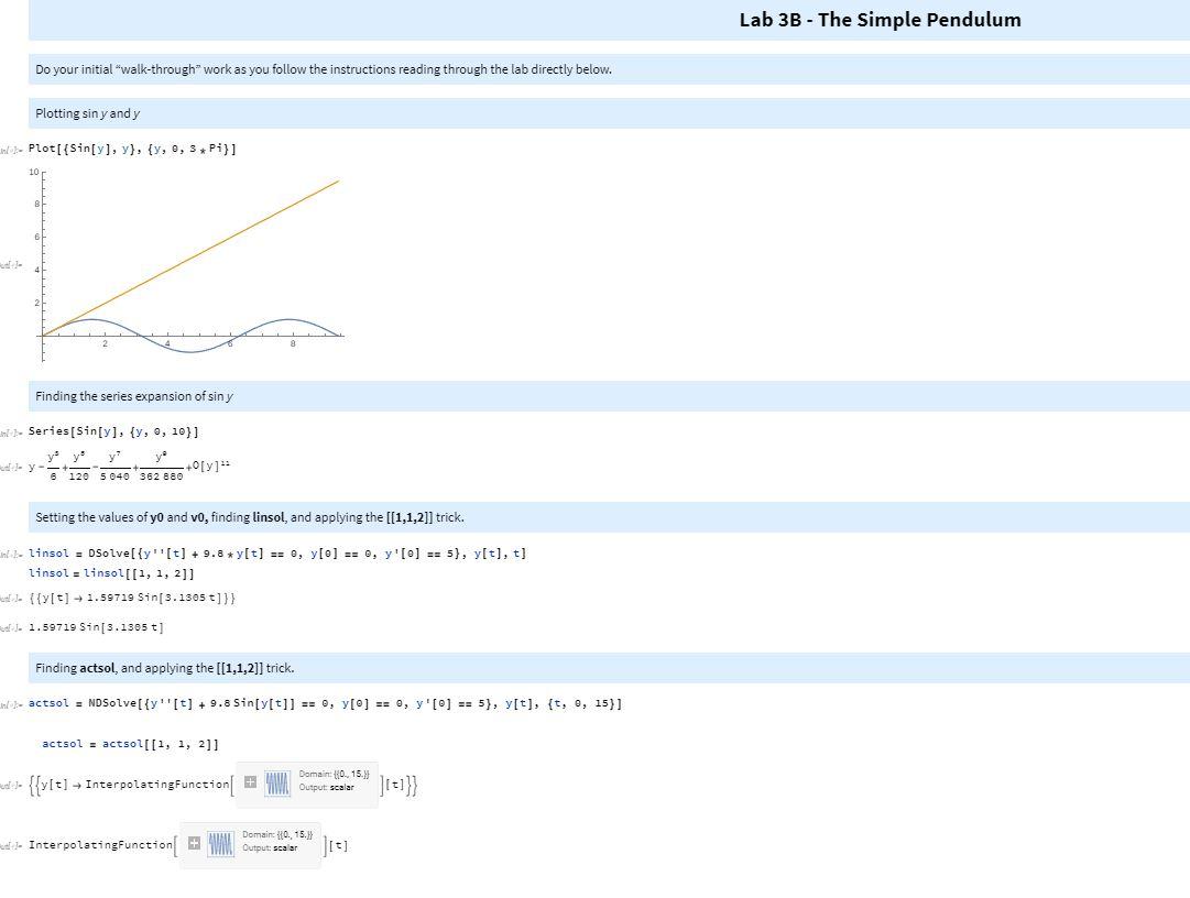
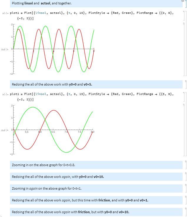
Lab 3B - The Simple Pendulum Do your initial "walk-through" work as you follow the instructions reading through the lab directly below. Plotting sin y and y ino). Plot[{Sin[y], y}, {y, 0, 3. Pi}] Finding the series expansion of siny Series (Sin[y], {y, 9, 10}] y yiyi y ly- 120 5040362 88 +0 [y]*- Setting the values of yo and vo, finding linsol, and applying the [[1,1,2]] trick. in 1- linsot = Dsolve[{y"[t] + 9.8 *y[t] == 0, y[0] == 0, y'[0] == 5), y(t), t] linsol = linsol[(1, 1, 2]] 1. {{y[t] + 1.59719 Sin (3.1505 t]}} af J. 1.59719 Sin[3.1305 t] Finding actsol, and applying the [[1,1,2]] trick. no actsol = NDSolve[{y''[t] + 9.8 Sin[y[t]] == 0, y[0] == 0, y '[0] == 5), y[t], {t, 0, 15}] actsol = actsol[[1, 1, 2]] wedst {{v[t] InterpolatingFunction Domain: 10.,15.) Output scalar - InterpolatingFunction + Domain 110. 15.) Output: scalar 1151 Plotting linsol and actsol, and together. intihaplota = Plot[{linsol, actsol}, {t, 0, 15), PlotStyle + {Red, Green), PlotRange + {{0, 8), 1-2, 2}}] DO Redoing the all of the above work with yo=0 and vo=5. MA ca in 1- ploti - Plot[{linsol, actsol}, {t, , 15), PlotStyle + {Red, Green), PlotRange + {{5, 8), {-2, 2}}] Dual - 0 5.5 6.5 7.0 75 90 Zooming in on the above graph for 0