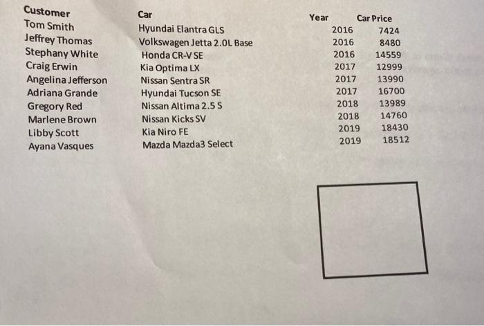
This practical test requires you to be able to manipulate your worksheet, to create formulas, to use relative and absolute addressing, to use functions: sum, max, min, average, count and if, to Sr create charts, and to format your worksheet. . 1. Download and save the file CasSales as YourNameCarSales.. During the process of your work save often to avoid losing your work. 2. In this file you are given information about car inventory of a dealership in New Britain. The dealership is providing financial assistance to its customers. 3. You can see information about the customer, the car, year of manufacturing and price of the car. You also have the following information: ----Cars manufactured in 2018 or after are getting 10% discount ----Cars, manufactured prior to 2018 aren't getting a discount. ---Sales tax in Connecticut is 6% -The dealership requires 5% down payment from the customers. -You are required to calculate the discount, price after discount, sales tax, down payment, and amount to finance. 4. Insert several rows at the beginnings of the worksheet and type in the title: Sales of Used Cars: Schaller, New Britain 5. Below the title type: Prepared by Your name 6. Two rows below your name enter the assumptions that you are going to use for the calculations. 7. Before the column Year of Manufacturing insert a column Color. 8. Enter the colors in the cells (black, red, white, silver- of your choice). 9. Create labels for the columns discount, price after discount, sales tax, down payment, and amount to finance 10. Using the appropriate formulas calculate the discount, price after discount, sales tax, down payment, and amount to finance. Use the information from your assumptions. 11. Using the appropriate functions calculate Maximum Car Price, Minimum Car Price, Average car price, and Number of cars in inventory. 12.Below the worksheet area calculate the totals for the car prices for Year 2016, Year2017, Year2018, and Year2019. 13. Create a pie chart for this information (year and car price). The chart should have a title: Total of Car Price for Years 2016-2019. Legend should be at the bottom of the chart. The data label should be displayed in the center of the pie segments. Move the pie chart to a new sheet and name it Cars Statistics. 14. Format nicely the worksheet using borders, shading, colors, and anything that is going to give a professional appearance. All values should be appropriately formatted as dollars. Save and submit. Customer Tom Smith Jeffrey Thomas Stephany White Craig Erwin Angelina Jefferson Adriana Grande Gregory Red Marlene Brown Libby Scott Ayana Vasques Car Hyundai Elantra GLS Volkswagen Jetta 2.0L Base Honda CR-V SE Kia Optima LX Nissan Sentra SR Hyundai Tucson SE Nissan Altima 2.5 S Nissan Kicks SV Kia Niro FE Mazda Mazda3 Select Year Car Price 2016 7424 2016 8480 2016 14559 2017 12999 2017 13990 2017 16700 2018 13989 2018 14760 2019 18430 2019 18512 This practical test requires you to be able to manipulate your worksheet, to create formulas, to use relative and absolute addressing, to use functions: sum, max, min, average, count and if, to Sr create charts, and to format your worksheet. . 1. Download and save the file CasSales as YourNameCarSales.. During the process of your work save often to avoid losing your work. 2. In this file you are given information about car inventory of a dealership in New Britain. The dealership is providing financial assistance to its customers. 3. You can see information about the customer, the car, year of manufacturing and price of the car. You also have the following information: ----Cars manufactured in 2018 or after are getting 10% discount ----Cars, manufactured prior to 2018 aren't getting a discount. ---Sales tax in Connecticut is 6% -The dealership requires 5% down payment from the customers. -You are required to calculate the discount, price after discount, sales tax, down payment, and amount to finance. 4. Insert several rows at the beginnings of the worksheet and type in the title: Sales of Used Cars: Schaller, New Britain 5. Below the title type: Prepared by Your name 6. Two rows below your name enter the assumptions that you are going to use for the calculations. 7. Before the column Year of Manufacturing insert a column Color. 8. Enter the colors in the cells (black, red, white, silver- of your choice). 9. Create labels for the columns discount, price after discount, sales tax, down payment, and amount to finance 10. Using the appropriate formulas calculate the discount, price after discount, sales tax, down payment, and amount to finance. Use the information from your assumptions. 11. Using the appropriate functions calculate Maximum Car Price, Minimum Car Price, Average car price, and Number of cars in inventory. 12.Below the worksheet area calculate the totals for the car prices for Year 2016, Year2017, Year2018, and Year2019. 13. Create a pie chart for this information (year and car price). The chart should have a title: Total of Car Price for Years 2016-2019. Legend should be at the bottom of the chart. The data label should be displayed in the center of the pie segments. Move the pie chart to a new sheet and name it Cars Statistics. 14. Format nicely the worksheet using borders, shading, colors, and anything that is going to give a professional appearance. All values should be appropriately formatted as dollars. Save and submit. Customer Tom Smith Jeffrey Thomas Stephany White Craig Erwin Angelina Jefferson Adriana Grande Gregory Red Marlene Brown Libby Scott Ayana Vasques Car Hyundai Elantra GLS Volkswagen Jetta 2.0L Base Honda CR-V SE Kia Optima LX Nissan Sentra SR Hyundai Tucson SE Nissan Altima 2.5 S Nissan Kicks SV Kia Niro FE Mazda Mazda3 Select Year Car Price 2016 7424 2016 8480 2016 14559 2017 12999 2017 13990 2017 16700 2018 13989 2018 14760 2019 18430 2019 18512