This question requires Matlab . A coding designed in fluid mechanics for the change in head loss per unit piple length as a function of flow rate . However the coding was designed to show the change for only one D value . Your job is to modify the coding to give a plot for 3 D values (0.025 ,0.05,0.075). They all need to be in the same graph . Just focus on the modifying the coding to accomadate three D values in the same plot . Also , a picture of the final result is attached . Make sure to get the same plot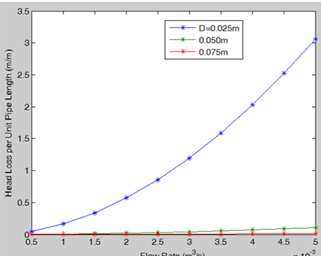

The coding (script file) is the follwing

function dummy %This allows you to pack everything into a single m-file

close all, clear all, clc, format compact %Clean up

global Re eoverD %To pass values to function below

e=1.5e-6; %roughness for drawn tubing

nu=6.58e-7; %kinematic viscosity

D=input('enter D values')

Q=linspace(5e-4, 50e-4, 10);

for i = 1:10

V=Q(i)/(0.25*pi*D^2);

eoverD=e/D; %relative roughness

Re=V*Du;

%Use Colebrook formula to get f with initial guess

f=fsolve(@colebrook, 0.02);

hLoverL(i)=f/D*V^2/2/9.81

end

plot (Q, hLoverL, 'o-r')

ylabel('\fontname{Arial} Heat Loss Per Unit Length (m/m)','Fontsize',12);

xlabel('\fontname{Arial}Flow Rate m^3/s','Fontsize',12);

function residual=colebrook(f) %fsolve will try to make residual=0

global Re eoverD

residual=1/sqrt(f)+2*log10(eoverD/3.7 + 2.51/Re/sqrt(f));

3.5 3 -. 0.075m s 2.5 2 1.5 0.5 0.5 1 1.5 2 2.5 3 3.5 4 455 5 3 3.5 3 -. 0.075m s 2.5 2 1.5 0.5 0.5 1 1.5 2 2.5 3 3.5 4 455 5 3