

Question: This two codes for Gradient Descent algorithm for two vectors the first code for visualizing in 3D AND the second visualizing the function in 2D
This two codes for Gradient Descent algorithm for two vectors
the first code for visualizing in 3D AND the second visualizing the function in 2D
I want to update these two codes in order to replace the exist function with sphere function
please give me excutable codes without error message with simple explanations since can understand your updated codes
***************************************************************************************************************************************
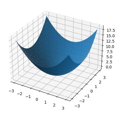
The first code :-
import numpy as np
from mpl_toolkits.mplot3d import Axes3D
import matplotlib.pyplot as plt
class GradientDescent:
def __init__(self, function, gradient, initial_solution, learning_rate=0.1, max_iter=100, tolerance=0.0000001):
self.function = function
self.gradient= gradient
self.solution = initial_solution
self.learning_rate = learning_rate
self.max_iter = max_iter
self.tolerance = tolerance
def run(self):
t = 0
while t
diff = -self.learning_rate*self.gradient(*self.solution)
if np.linalg.norm(diff)
break
self.solution += diff
t += 1
return self.solution, self.function(*self.solution)
def fun2(x, y):
return x**2 + y**2
def gradient2(x, y):
return np.array([2*x, 2*y])
bounds = [-3, 3]
fig = plt.figure()
ax = fig.add_subplot(111, projection='3d')
X = np.linspace(bounds[0], bounds[1], 100)
Y = np.linspace(bounds[0], bounds[1], 100)
X, Y = np.meshgrid(X, Y)
Z = fun2(X, Y)
ax.plot_surface(X, Y, Z)
random_solution = np.random.uniform(bounds[0], bounds[1], size=2)
gd = GradientDescent(fun2, gradient2, random_solution)
best_solution, best_value = gd.run()
ax.scatter(best_solution[0], best_solution[1], best_value, color='r', s=100)
plt.show()
***********************************************************************************************************
The second code :-
import numpy as np from matplotlib import pyplot as plt
class GradientDescent: def __init__(self, function, gradient, initial_solution, learning_rate=0.1, max_iter=100, tolerance=0.0000001): self.function = function self.gradient = gradient self.solution = initial_solution self.learning_rate = learning_rate self.max_iter = max_iter self.tolerance = tolerance
def run(self): t = 0 while t
def fun1(x, y): return x ** 2 + y ** 2
def gradient1(x, y): return np.array([2 * x, 2 * y])
bounds = [-3, 3]
plt.figure()
x, y = np.meshgrid(np.linspace(bounds[0], bounds[1], 100), np.linspace(bounds[0], bounds[1], 100)) z = fun1(x, y) plt.contour(x, y, z,levels=20)
random_solution = np.random.uniform(bounds[0], bounds[1], size=2)
gd = GradientDescent(fun1, gradient1, random_solution)
best_solution, best_value = gd.run()
plt.plot(best_solution[0], best_solution[1], marker='o') plt.plot(best_solution[0], best_solution[1])
plt.show() 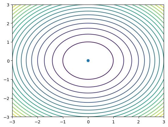
Step by Step Solution
There are 3 Steps involved in it

Get step-by-step solutions from verified subject matter experts