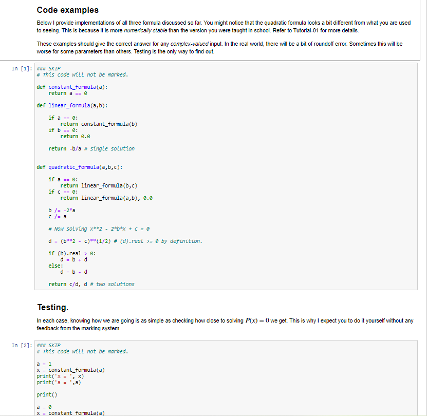
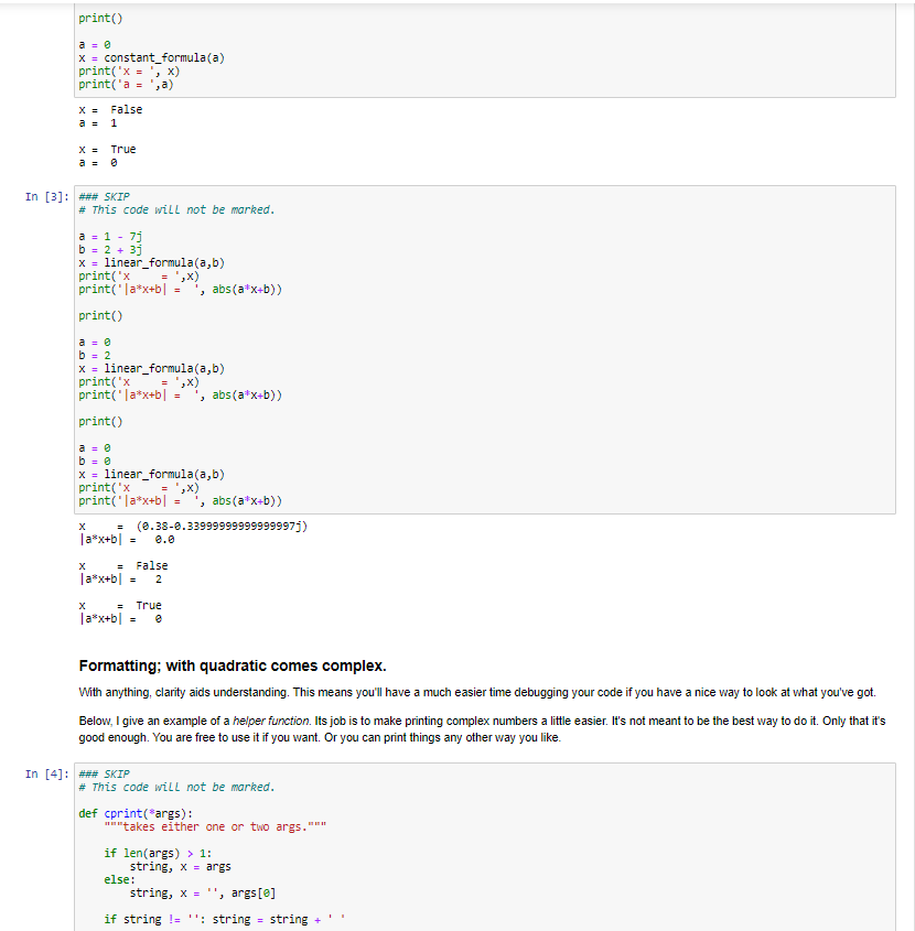
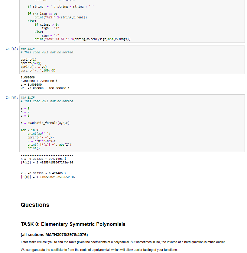
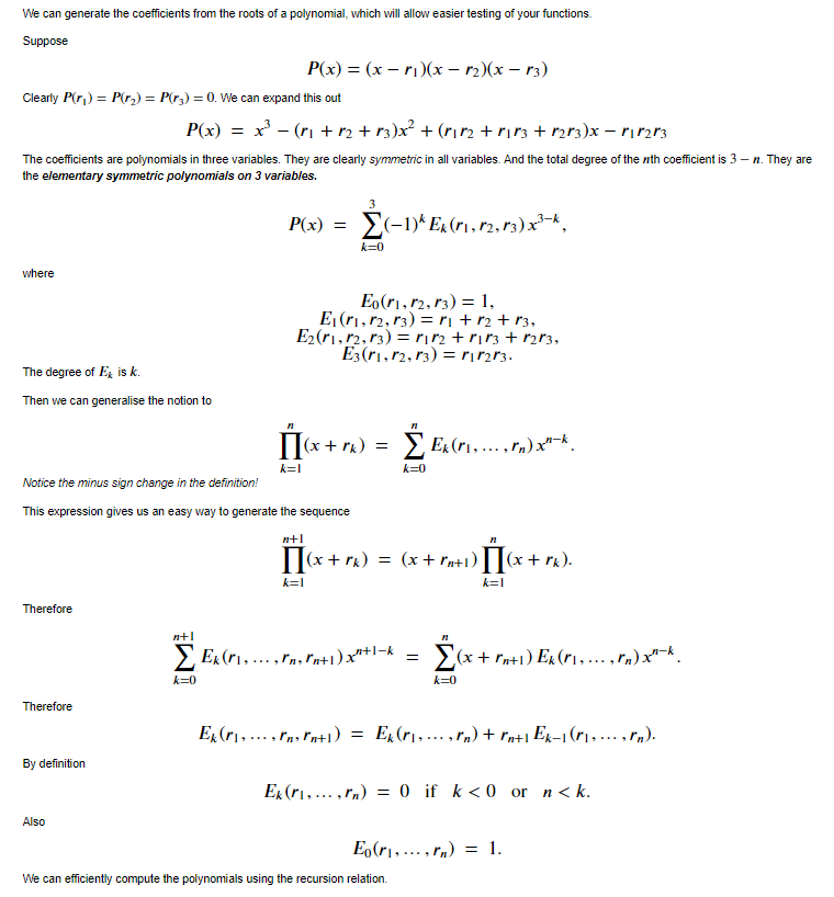
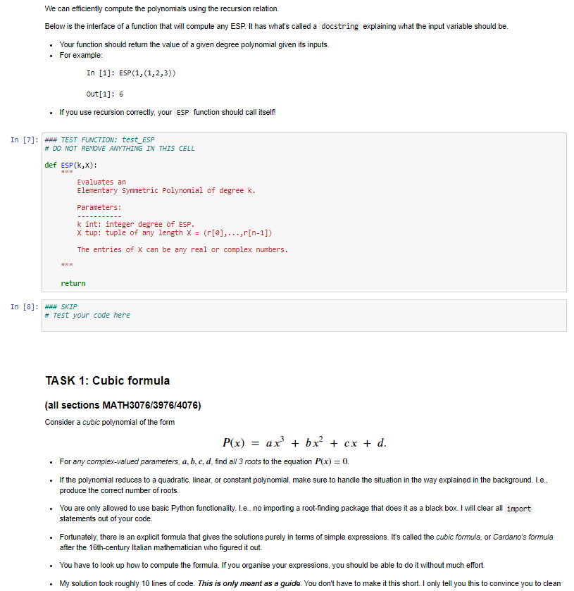
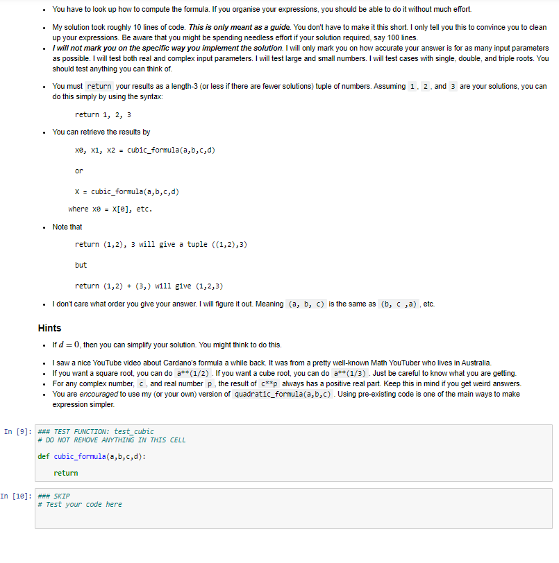
To practice basic Python programming of control and data structures. Spend time testing and debugging your work. Get experience looking up background material on the Internet. For the 1st item, you will only be allowed to use Basic Python functionality. What does this mean? Built-in syntax, e.g., function definitions, if statements, and basic numerical operators like .real, .imag No import statements of any kind, i.e., no libraries. I will clear any imported libraries before marking. For the 2nd item, you will need to test your output very carefully. What does this mean? For the problems given, you can easily check if your results are correct. If (when) your results do not behave as you expect, you will need to include lots of print statements inside your functions to see what's going wrong. Experience shows that students are reluctant to "dive in" to debugging. I think the reason for this is familiarity with paper mathematics, where there is no easy from the equations to talk back to you. Checking an answer can be time-consuming. With code, you are making progress as long as you are typing something Some of you may have experience where the "Mark" or "Submit" button tells you if you have the right solutions on ED. I might do this in the future. Not for this assignment. For this assignment, you have all the tools needed to determine if your answers are correct or not. I want you to worry about your answers being not correct. NASA just landed a car and a helicopter on Mars. They didn't have a "mark" button that told them if their spaceship would crash or not. They landed successfully because they checked their answers carefully. For the 3rd item, you will need to teach yourself the required formulas from Internet (or book) resources. What does that mean? There are numerous YouTube videos explaining exactly how to compute the required functions. There are also extensive Wikipedia pages on Cardano's and Ferrari's methods. That should be enough of a hint to find lots of other examples. A challenge of this assignment is that there are many equivalent looking formulas that don't always work the same way. You will need to test different things out. A bit of background Quadratic formula You all know the quadratic formula. It was first discovered 5000 years ago. That is consider a quadratic polynomial of the form P(x) = ax + bx + c. The roots of the equation P(x) = 0 satisfy the formula "by radicals" 2 X = b 2a + - C. Moreover, the formula works for any complex-valued parameters, a,b,c. We can see there is no problem as long as a = 0. If the leading-order coefficient does vanish, then the polynomial is not quadratic. It is only linear. Linear formula If the polynomial is of the form P(x) = ax + b Then the roots are even easier Then the roots are even easier, b x = a x = Like before, this is valid provided a 70. Should we stop here, or is there an even simpler situation? Constant formula If the leading-order coefficient of a linear function vanishes, then the "polynomial" is a constant function P(x) = a. Now there are only two possible cases for the "roots". If a #0, there are no roots. If a = 0, then any number is a root. That is, None a +0 Everything a = 0. Perhaps a good way to express None and Everything is with False and True. We can think of them as either synonyms, or encodings. But just going with it, S False a 80 True a=0. But this is identical to the logical statement x = (a == 0). At this point, we are totally done. There is no more bottom level to consider. X = Why the level of detail? Hopefully, you realise that we won't usually worry quite so much about the "trivial" things like "solving for the roots of a constant function". It's all meant for illustration. Normally you will write code for some well-understood set of operating parameters, and anything outside those parameters will throw an error and cause the program to stop. But there are both practical and philosophical reasons for getting to the bottom of everything. The most practical reason for avoiding error is so you can test for problems and correct them without killing your program. This is what professionals often do when writing mission-critical code. There are also philosophical and pedagogical reasons for spelling it out. What is the moral of the story? There are several: Did you notice that I reused the letters a, b? They meant different things in different contexts. But I'm guessing you didn't get confused. Math is like this, and code has good ways of reflecting it. That's the idea of the environment, or namespace. Did you get the sense that the math was creating a descending hierarchy of more specific cases that sort of build on each other? Math is like this, and code has good ways of reflecting it. This is the hierarchal and modular programming. Did you notice how the mathematical expression required the use of" if statements" to make full sense of the situation. Math is like this, and code has good ways of reflecting it. That's the idea of control structures. Did you notice the base case ended not with numbers but more abstract ideas such as "None" and "Alt"? Math and Life are often like that. Once you get really far down, you run into quite simple and quite strange things all the same time. This is a good indication that you've hit bottom. It also clarifies that math, calculations, and code are here for the benefit of humans, so it should be no surprise that it sometimes gives human-type responses. And for humans to make decisions, there is nothing more useful than "True" and "False". Code examples Below I provide implementations of all three formula discussed so far. You might notice that the quadratic formula looks a bit different from what you are used to seeing. This is because it is more numerically stable than the version you were taught in school. Refer to Tutorial-01 for more details. These examples should give the correct answer for any complex-valued input. In the real world, there will be a bit of roundoff error. Sometimes this will be worse for some parameters than others. Testing is the only way to find out. In [1]: *** SKIP # This code will not be marked. def constant_formula(a): return a us @ def linear_formula(a,b): if a = 2: return constant_formula(b) if b == e: return 0.0 return -b/a # single solution def quadratic_formula(a,b,c): if a = @: return linear_formula(b, c) if c = @: return linear_formula(a,b), 0.0 b/= -28a c/= a # Now solving x**2 - 2*b*x + C = 8 da (b**2 - )** (1/2) # (d).real >= @by definition. if (b).real > : d = b + d else: d = b - d return c/d, d # two solutions Testing. In each case, knowing how we are going is as simple as checking how close to solving P(x) = 0 we get. This is why I expect you to do it yourself without any feedback from the marking system. In [2]: #*# SKIP # This code will not be marked. a = 1 X = constant_formula(a) print('x = ',x) print('a = ',a) print() X = constant formula(a) print X = constant_formula(a) print('x = ',x) print('a = 'ja) X = False a = 1 X = True In [3]: ### SKIP # This code will not be marked. a = 1 - 7 b = 2 + 3) x = linear_formula(a,b) print('x = ',x) print('|a*x+b] , abs(a*x+b)) print() b = 2 x = linear_formula(a,b) print('x = ',x) print('|a*x+b] = , abs(a*x+b)) printo x = linear_formula(a,b) print("x = ',x) print('la*x+b = , abs(a*x+b)) (0.38-0.339999999999999971) 1a*x+b = False | a*x+b] = 2 2 True la*x+b] = e Formatting; with quadratic comes complex. With anything, clarity aids understanding. This means you'll have a much easier time debugging your code if you have a nice way to look at what you've got. Below, I give an example of a helper function. Its job is to make printing complex numbers a little easier. It's not meant to be the best way to do it. Only that it's good enough. You are free to use it if you want. Or you can print things any other way you like. In [4]: ### SKIP # This code will not be marked. def cprint("args): takes either one or two args. if len(args) > 1: string, X = args else: string, X = , args[e] if string != ''; string = string + if string != ''; string = string + if (x). imag print("%s%f" %(string,x.real)) else: if x.image: sign = "" else: sign = print("%s%f %s %f i" %(string,x.real, sign, abs(x.imag))) In [5]: ### SKIP # This code will not be marked. cprint(1) cprint(5+71) cprint('z =',5) cprint('w: ',1883-3) 1.eeeeee 5.820080 + 7.000000 i z = 5.820000 W: -3.eeeeee + 100.eeeeee i In [6]: *** SKIP # This code will not be marked. b = 2 C = 1 X = quadratic_formula(a,b,c) for x in X: print(30*'-') cprint("x = ',x) Z = a*x**2+bx+c print("P(x) =', abs(z)) print) X = -0.333333 + 2.471405 i |P(x) = 2.4825341532472732-16 x = -0.333333 -0.471405 i |P(x) = 1.1102230246251565e-16 Questions TASK O: Elementary Symmetric Polynomials (all sections MATH3076/3976/4076) Later tasks will ask you to find the roots given the coefficients of a polynomial. But sometimes in life, the inverse of a hard question is much easier. We can generate the coefficients from the roots of a polynomial, which will allow easier testing of your functions. We can generate the coefficients from the roots of a polynomial, which will allow easier testing of your functions. Suppose P(x) = (x - n1)(x - 2)(x r3) Clearly Pri) = P(r) = P(r3) = 0. We can expand this out P(x) = x? - (n + 12 +13)x + (1112 +r113 + n2r3)x - r1 r2r3 The coefficients are polynomials in three variables. They are clearly symmetric in all variables. And the total degree of the nth coefficient is 3 - n. They are the elementary symmetric polynomials on 3 variables. 3 P(x) = (-1)* Ex (11,12,13) x3-k, 11,12 k=0 where Eo(ri,12,13) = 1, Eiri,12,13) = r + r2 + 13, E2(11,12,13) = rn2+ r13 + 1213, Ez(ri,12,13) = r2r3. The degree of Exis k. Then we can generalise the notion to [[(x+ru) = Ex(r...,) x**. k=0 k=I Notice the minus sign change in the definition! This expression gives us an easy way to generate the sequence n+! 11(x+r) = (x + Pn+1) (x + r). k=1 k=1 Therefore n+1 Ex(", ..., In, Pn+1)x*+1-k = (x +rn+1) Ex(n.... ,!m).xn-k. k=0 k=0 Therefore Ex(r. ..., r'n Pn+1) = Ex(11,..., rn) +rn+iEx-1(1, ... ,In). By definition Ex(r1, ... , In) = 0 if k= @by definition. if (b).real > : d = b + d else: d = b - d return c/d, d # two solutions Testing. In each case, knowing how we are going is as simple as checking how close to solving P(x) = 0 we get. This is why I expect you to do it yourself without any feedback from the marking system. In [2]: #*# SKIP # This code will not be marked. a = 1 X = constant_formula(a) print('x = ',x) print('a = ',a) print() X = constant formula(a) print X = constant_formula(a) print('x = ',x) print('a = 'ja) X = False a = 1 X = True In [3]: ### SKIP # This code will not be marked. a = 1 - 7 b = 2 + 3) x = linear_formula(a,b) print('x = ',x) print('|a*x+b] , abs(a*x+b)) print() b = 2 x = linear_formula(a,b) print('x = ',x) print('|a*x+b] = , abs(a*x+b)) printo x = linear_formula(a,b) print("x = ',x) print('la*x+b = , abs(a*x+b)) (0.38-0.339999999999999971) 1a*x+b = False | a*x+b] = 2 2 True la*x+b] = e Formatting; with quadratic comes complex. With anything, clarity aids understanding. This means you'll have a much easier time debugging your code if you have a nice way to look at what you've got. Below, I give an example of a helper function. Its job is to make printing complex numbers a little easier. It's not meant to be the best way to do it. Only that it's good enough. You are free to use it if you want. Or you can print things any other way you like. In [4]: ### SKIP # This code will not be marked. def cprint("args): takes either one or two args. if len(args) > 1: string, X = args else: string, X = , args[e] if string != ''; string = string + if string != ''; string = string + if (x). imag print("%s%f" %(string,x.real)) else: if x.image: sign = "" else: sign = print("%s%f %s %f i" %(string,x.real, sign, abs(x.imag))) In [5]: ### SKIP # This code will not be marked. cprint(1) cprint(5+71) cprint('z =',5) cprint('w: ',1883-3) 1.eeeeee 5.820080 + 7.000000 i z = 5.820000 W: -3.eeeeee + 100.eeeeee i In [6]: *** SKIP # This code will not be marked. b = 2 C = 1 X = quadratic_formula(a,b,c) for x in X: print(30*'-') cprint("x = ',x) Z = a*x**2+bx+c print("P(x) =', abs(z)) print) X = -0.333333 + 2.471405 i |P(x) = 2.4825341532472732-16 x = -0.333333 -0.471405 i |P(x) = 1.1102230246251565e-16 Questions TASK O: Elementary Symmetric Polynomials (all sections MATH3076/3976/4076) Later tasks will ask you to find the roots given the coefficients of a polynomial. But sometimes in life, the inverse of a hard question is much easier. We can generate the coefficients from the roots of a polynomial, which will allow easier testing of your functions. We can generate the coefficients from the roots of a polynomial, which will allow easier testing of your functions. Suppose P(x) = (x - n1)(x - 2)(x r3) Clearly Pri) = P(r) = P(r3) = 0. We can expand this out P(x) = x? - (n + 12 +13)x + (1112 +r113 + n2r3)x - r1 r2r3 The coefficients are polynomials in three variables. They are clearly symmetric in all variables. And the total degree of the nth coefficient is 3 - n. They are the elementary symmetric polynomials on 3 variables. 3 P(x) = (-1)* Ex (11,12,13) x3-k, 11,12 k=0 where Eo(ri,12,13) = 1, Eiri,12,13) = r + r2 + 13, E2(11,12,13) = rn2+ r13 + 1213, Ez(ri,12,13) = r2r3. The degree of Exis k. Then we can generalise the notion to [[(x+ru) = Ex(r...,) x**. k=0 k=I Notice the minus sign change in the definition! This expression gives us an easy way to generate the sequence n+! 11(x+r) = (x + Pn+1) (x + r). k=1 k=1 Therefore n+1 Ex(", ..., In, Pn+1)x*+1-k = (x +rn+1) Ex(n.... ,!m).xn-k. k=0 k=0 Therefore Ex(r. ..., r'n Pn+1) = Ex(11,..., rn) +rn+iEx-1(1, ... ,In). By definition Ex(r1, ... , In) = 0 if k