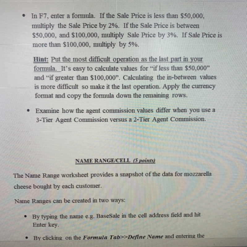
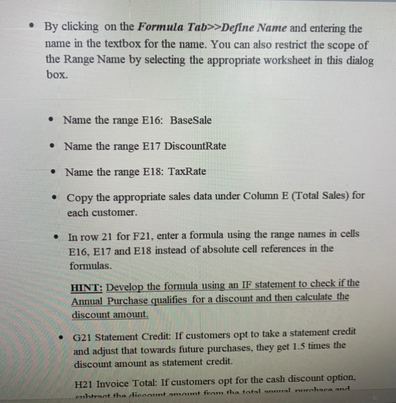
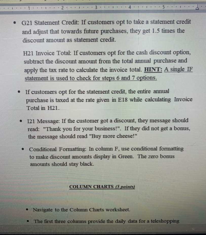
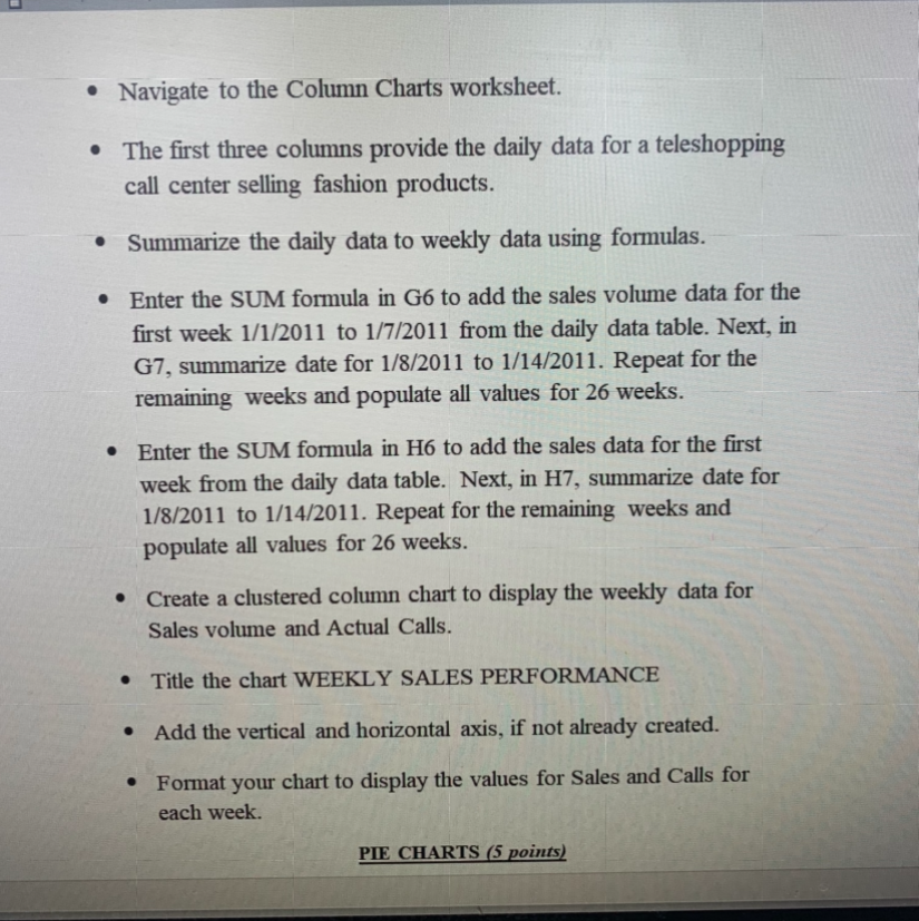
Topics covered COLUMN CHART, PIE CHART, IF FORMULA, NESTED IF FORMULA NAME RANGE/CELL and CONDITIONAL CELL FORMATTING IF and Nested IF (5 points) Watch all assigned videos especially for the IF and Nested functions since most students struggle with these formulas. . Examine the Assignment details worksheet and enter your full name. Click on the Customer Relations worksheet and play around with the data by sorting, filtering etc. Use various filtering options such as text options. Remove all filters and sort data based on Order date. Click on the IF & Nested IF sheet: In E6, enter the column heading 2-Tier Commission. In E7, enter a formula. If the Sale Price is at least $50,000, multiply the Sale Price by 5%, otherwise multiple Sale Price by 2%. Apply the currency format and copy the formula down the remaining rows. In F6, enter the column heading 3-Tier Commission. Resize your column suitably In F7, enter a formula. If the Sale Price is less than $50,000, multiply the Sale Price by 2%. If the Sale Price is between $50,000, and $100,000, multiply Sale Price by 3%. If Sale Price is more than $100,000, multiply by 5%. Hint: Put the most difficult operation as the last part in your formula. _It's easy to calculate values for if less than $50,000" and if greater than $100,000. Calculating the in-between values is more difficult so make it the last operation. Apply the currency format and copy the formula down the remaining rows. Examine how the agent commission values differ when you use a 3-Tier Agent Commission versus a 2-Tier Agent Commission. NAME RANGE/CELL (5 points) The Name Range worksheet provides a snapshot of the data for mozzarella cheese bought by each customer. Name Ranges can be created in two ways: By typing the name e.g. BaseSale in the cell address field and hit Enter key. By clicking on the Formula Tab>>Define Name and entering the By clicking on the Formula Tab>>Define Name and entering the name in the textbox for the name. You can also restrict the scope of the Range Name by selecting the appropriate worksheet in this dialog box. Name the range E16: BaseSale Name the range E17 DiscountRate Name the range E18: TaxRate Copy the appropriate sales data under Column E (Total Sales) for each customer. In row 21 for F21, enter a formula using the range names in cells E16, E17 and E18 instead of absolute cell references in the formulas. HINT: Develop the formula using an IF statement to check if the Annual Purchase qualifies for a discount and then calculate the discount amount. G21 Statement Credit: If customers opt to take a statement credit and adjust that towards future purchases, they get 1.5 times the discount amount as statement credit. H21 Invoice Total: If customers opt for the cash discount option, cnhtract the discount amount from the total annual muchaca and 3 5 G21 Statement Credit: If customers opt to take a statement credit and adjust that towards future purchases, they get 1.5 times the discount amount as statement credit. H21 Invoice Total: If customers opt for the cash discount option, subtract the discount amount from the total annual purchase and apply the tax rate to calculate the invoice total. HINT: A single IF statement is used to check for steps 6 and 7 options. If customers opt for the statement credit, the entire annual purchase is taxed at the rate given in E18 while calculating Invoice Total in H21. 121 Message: If the customer got a discount, they message should read: "Thank you for your business!". If they did not get a bonus, the message should read "Buy more cheese!" Conditional Formatting: In column F, use conditional formatting to make discount amounts display in Green. The zero bonus amounts should stay black. COLUMN CHARTS (5 points) Navigate to the Column Charts worksheet. The first three columns provide the daily data for a teleshoppin Navigate to the Column Charts worksheet. The first three columns provide the daily data for a teleshopping call center selling fashion products. Summarize the daily data to weekly data using formulas. Enter the SUM formula in G6 to add the sales volume data for the first week 1/1/2011 to 1/7/2011 from the daily data table. Next, in G7, summarize date for 1/8/2011 to 1/14/2011. Repeat for the remaining weeks and populate all values for 26 weeks. Enter the SUM formula in H6 to add the sales data for the first week from the daily data table. Next, in H7, summarize date for 1/8/2011 to 1/14/2011. Repeat for the remaining weeks and populate all values for 26 weeks. Create a clustered column chart to display the weekly data for Sales volume and Actual Calls. Title the chart WEEKLY SALES PERFORMANCE Add the vertical and horizontal axis, if not already created. Format your chart to display the values for Sales and Calls for each week. PIE CHARTS (5 points) Title the chart WEEKLY SALES PERFORMANCE Add the vertical and horizontal axis, if not already created. Format your chart to display the values for Sales and Calls for each week. PIE CHARTS (5 points) Click on the Pie Charts worksheet Create a 3D-Pie chart of the products purchased by Bert's Bistro using the Product Name and Total Cost columns. O Format the legend appropriately if required. Add the Data Labels to show the amount Format the data labels to display both amount and percentage. Title the chart Bert's Bistro Purchases. Position the chart in E18:K36. Submission Instructions: Name your file as your LastName_FirstName Excel-3.xlsx and submit on Blackboard. Topics covered COLUMN CHART, PIE CHART, IF FORMULA, NESTED IF FORMULA NAME RANGE/CELL and CONDITIONAL CELL FORMATTING IF and Nested IF (5 points) Watch all assigned videos especially for the IF and Nested functions since most students struggle with these formulas. . Examine the Assignment details worksheet and enter your full name. Click on the Customer Relations worksheet and play around with the data by sorting, filtering etc. Use various filtering options such as text options. Remove all filters and sort data based on Order date. Click on the IF & Nested IF sheet: In E6, enter the column heading 2-Tier Commission. In E7, enter a formula. If the Sale Price is at least $50,000, multiply the Sale Price by 5%, otherwise multiple Sale Price by 2%. Apply the currency format and copy the formula down the remaining rows. In F6, enter the column heading 3-Tier Commission. Resize your column suitably In F7, enter a formula. If the Sale Price is less than $50,000, multiply the Sale Price by 2%. If the Sale Price is between $50,000, and $100,000, multiply Sale Price by 3%. If Sale Price is more than $100,000, multiply by 5%. Hint: Put the most difficult operation as the last part in your formula. _It's easy to calculate values for if less than $50,000" and if greater than $100,000. Calculating the in-between values is more difficult so make it the last operation. Apply the currency format and copy the formula down the remaining rows. Examine how the agent commission values differ when you use a 3-Tier Agent Commission versus a 2-Tier Agent Commission. NAME RANGE/CELL (5 points) The Name Range worksheet provides a snapshot of the data for mozzarella cheese bought by each customer. Name Ranges can be created in two ways: By typing the name e.g. BaseSale in the cell address field and hit Enter key. By clicking on the Formula Tab>>Define Name and entering the By clicking on the Formula Tab>>Define Name and entering the name in the textbox for the name. You can also restrict the scope of the Range Name by selecting the appropriate worksheet in this dialog box. Name the range E16: BaseSale Name the range E17 DiscountRate Name the range E18: TaxRate Copy the appropriate sales data under Column E (Total Sales) for each customer. In row 21 for F21, enter a formula using the range names in cells E16, E17 and E18 instead of absolute cell references in the formulas. HINT: Develop the formula using an IF statement to check if the Annual Purchase qualifies for a discount and then calculate the discount amount. G21 Statement Credit: If customers opt to take a statement credit and adjust that towards future purchases, they get 1.5 times the discount amount as statement credit. H21 Invoice Total: If customers opt for the cash discount option, cnhtract the discount amount from the total annual muchaca and 3 5 G21 Statement Credit: If customers opt to take a statement credit and adjust that towards future purchases, they get 1.5 times the discount amount as statement credit. H21 Invoice Total: If customers opt for the cash discount option, subtract the discount amount from the total annual purchase and apply the tax rate to calculate the invoice total. HINT: A single IF statement is used to check for steps 6 and 7 options. If customers opt for the statement credit, the entire annual purchase is taxed at the rate given in E18 while calculating Invoice Total in H21. 121 Message: If the customer got a discount, they message should read: "Thank you for your business!". If they did not get a bonus, the message should read "Buy more cheese!" Conditional Formatting: In column F, use conditional formatting to make discount amounts display in Green. The zero bonus amounts should stay black. COLUMN CHARTS (5 points) Navigate to the Column Charts worksheet. The first three columns provide the daily data for a teleshoppin Navigate to the Column Charts worksheet. The first three columns provide the daily data for a teleshopping call center selling fashion products. Summarize the daily data to weekly data using formulas. Enter the SUM formula in G6 to add the sales volume data for the first week 1/1/2011 to 1/7/2011 from the daily data table. Next, in G7, summarize date for 1/8/2011 to 1/14/2011. Repeat for the remaining weeks and populate all values for 26 weeks. Enter the SUM formula in H6 to add the sales data for the first week from the daily data table. Next, in H7, summarize date for 1/8/2011 to 1/14/2011. Repeat for the remaining weeks and populate all values for 26 weeks. Create a clustered column chart to display the weekly data for Sales volume and Actual Calls. Title the chart WEEKLY SALES PERFORMANCE Add the vertical and horizontal axis, if not already created. Format your chart to display the values for Sales and Calls for each week. PIE CHARTS (5 points) Title the chart WEEKLY SALES PERFORMANCE Add the vertical and horizontal axis, if not already created. Format your chart to display the values for Sales and Calls for each week. PIE CHARTS (5 points) Click on the Pie Charts worksheet Create a 3D-Pie chart of the products purchased by Bert's Bistro using the Product Name and Total Cost columns. O Format the legend appropriately if required. Add the Data Labels to show the amount Format the data labels to display both amount and percentage. Title the chart Bert's Bistro Purchases. Position the chart in E18:K36. Submission Instructions: Name your file as your LastName_FirstName Excel-3.xlsx and submit on Blackboard