use Python

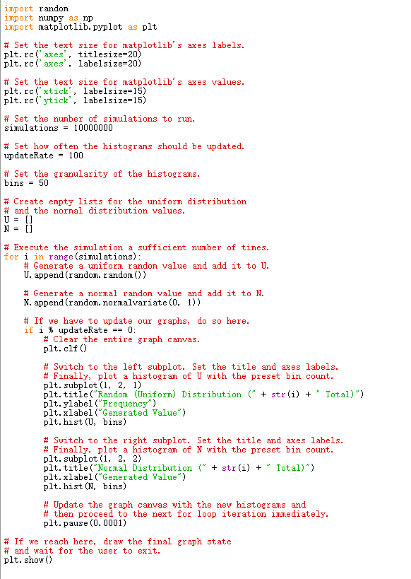
In this lab you will estimate probabilities using a Monte Carlo simulation. Implement the bisection algorithm for finding the roots (zeros) of a function. (1) (a) Write and test a Boolean function: hasComplexRoots (a, b, c), that returns True if the quadratic ar+bx+c=0 has em complex roots and False otherwise. -b + b2 - 4ac Note: The roots of the quadratic above are given by x = 2a (b) Using the function hasComplexRoots(a, b, c), to compute the probability Pi (n) (the Monte Carlo estimate) that the quadratic has complex roots, assuming that the coefficients are drawn from a uniform random distribution on [0,1], (using random.random()). Run the simulation for n = 1000. Repeat the experiment to compute P2(n), where the coefficients are chosen from a normal distribution (random.normalvariate(0, 1)) with mean mu = 0 and std. deviation sigma = 1. (2) Implement a function bisection, that can operate on an arbitrary function. Your program should accept: a function (f - to find the roots/zeros of); two endpoints (x0, xl); a tolerance limit (e) and the max. number of iterations n as input parameters. The function bisection should output the final approxima- tion to the root (zero) and the number of iterations it took to find the root. The program should make sure that the initial interval is acceptable for this method (i.e. (1) it should be greater than the tolerance () and (ii) must contain a zero of f (i.e. f(x0) f(xl) In 2 Set this value as your max. iterations m. The bisection method for finding roots was covered in class. The algorithm is in the notes on-line. . Notel: Define Python functions for function evaluations in the problems: Note2: You can return two values from a python function using return rootApprox, iterCount as the final line in the function. Make sure to pick up both values in the calling code as: xr, numIter = bisection(a, b, tol, f) for example. Use the bisection(f, x0, x1, tol, m) to compute (i) the positive root of f(x) = x2 1 1. The positive root of this equation is known to lie in the interval [1,2]. Use a tolerance of f 10-8. (ii) Repeat this exercise for the negative root:. Search in (-1,0). (The solution to (i) is the Golden Ratio: o the limit of the ratio of consecutive Fibonacci numbers. The solution to (ii) is known to be -1/9). Use your program to compute the roots of f(t) = x3 3.0 - 1 on [0, 1], f2() = 2 sin(t) on (0.5, 2], f3 = tan() 2.c on [0, 2). Start by plotting the functions to find a reasonable interval to bracket the root and print x, f(t) and the number of iterations required for convergence. import random import nupy as np import matplotlib. pyplot as plt # Set the text size for matplotlib's axes labels. plt. rc('axes", titlesize=20) plt. rc(' axes', labelsize=20) # Set the text size for matplotlib's axes values. plt. rc('xtick, labelsize=15) plt.rc('ytick', labelsize=15) # Set the number of simulations to run. simulations = 10000000 # Set how often the histograms should be updated. updateRate = 100 # Set the granularity of the histograms. bins = 50 # Create empty lists for the uniform distribution # and the normal distribution values. U = [] N = [] # Execute the simulation a sufficient number of times. for i in range (simulations): # Generate a uniform random value and add it to U. U. append(random. random()) # Generate a normal random value and add it to N. N. append(random. normalvariate(0, 1)) # If we have to update our graphs, do so here. if i % updateRate == 0: # Clear the entire graph canvas. plt.clf() # Switch to the left subplot. Set the title and axes labels. # Finally, plot a histogram of U with the preset bin count. plt. subplot (1, 2, 1) plt.title("Random (Uniform) Distribution (" + str(i) + Total)") plt. ylabel("Frequency") plt.xlabel("Generated Value") plt.hist (U, bins) # Switch to the right subplot. Set the title and axes labels. # Finally, plot a histogram of N with the preset bin count. plt. subplot(1, 2, 2) plt.title("Normal Distribution (" + str(i) + Total)") plt.xlabel("Generated Value") plt.hist (N, bins) # Update the graph canvas with the new histograms and # then proceed to the next for loop iteration immediately. plt.pause (0.0001) # If we reach here, draw the final graph state # and wait for the user to exit. plt.show()