Use R programming to answer following questions. Submit related R codes and outputs. Explain the results in your own words to answer each problem. The quality of Pinot Noir wine is thought to be related to the properties of clarity, aroma, body, flavor, and oakiness. Data for 38 wines are given in winequality.txt. Use read.csv("winequality.txt", sep="") to import the data.

"Clarity" "Aroma" "Body" "Flavor" "Oakiness" "Quality" "1" 1 3.3 2.8 3.1 4.1 9.8 "2" 1 4.4 4.9 3.5 3.9 12.6 "3" 1 3.9 5.3 4.8 4.7 11.9 "4" 1 3.9 2.6 3.1 3.6 11.1 "5" 1 5.6 5.1 5.5 5.1 13.3 "6" 1 4.6 4.7 5 4.1 12.8 "7" 1 4.8 4.8 4.8 3.3 12.8 "8" 1 5.3 4.5 4.3 5.2 12 "9" 1 4.3 4.3 3.9 2.9 13.6 "10" 1 4.3 3.9 4.7 3.9 13.9 "11" 1 5.1 4.3 4.5 3.6 14.4 "12" 0.5 3.3 5.4 4.3 3.6 12.3 "13" 0.8 5.9 5.7 7 4.1 16.1 "14" 0.7 7.7 6.6 6.7 3.7 16.1 "15" 1 7.1 4.4 5.8 4.1 15.5 "16" 0.9 5.5 5.6 5.6 4.4 15.5 "17" 1 6.3 5.4 4.8 4.6 13.8 "18" 1 5 5.5 5.5 4.1 13.8 "19" 1 4.6 4.1 4.3 3.1 11.3 "20" 0.9 3.4 5 3.4 3.4 7.9 "21" 0.9 6.4 5.4 6.6 4.8 15.1 "22" 1 5.5 5.3 5.3 3.8 13.5 "23" 0.7 4.7 4.1 5 3.7 10.8 "24" 0.7 4.1 4 4.1 4 9.5 "25" 1 6 5.4 5.7 4.7 12.7 "26" 1 4.3 4.6 4.7 4.9 11.6 "27" 1 3.9 4 5.1 5.1 11.7 "28" 1 5.1 4.9 5 5.1 11.9 "29" 1 3.9 4.4 5 4.4 10.8 "30" 1 4.5 3.7 2.9 3.9 8.5 "31" 1 5.2 4.3 5 6 10.7 "32" 0.8 4.2 3.8 3 4.7 9.1 "33" 1 3.3 3.5 4.3 4.5 12.1 "34" 1 6.8 5 6 5.2 14.9 "35" 0.8 5 5.7 5.5 4.8 13.5 "36" 0.8 3.5 4.7 4.2 3.3 12.2 "37" 0.8 4.3 5.5 3.5 5.8 10.3 "38" 0.8 5.2 4.8 5.7 3.5 13.2

Answers so far for reference:

R codes and output:

> d=read.table('data.txt',header=T,sep='')

> head(d)

Clarity Aroma Body Flavor Oakiness Quality

1 1 3.3 2.8 3.1 4.1 9.8

2 1 4.4 4.9 3.5 3.9 12.6

3 1 3.9 5.3 4.8 4.7 11.9

4 1 3.9 2.6 3.1 3.6 11.1

5 1 5.6 5.1 5.5 5.1 13.3

6 1 4.6 4.7 5.0 4.1 12.8

> attach(d)

The following objects are masked from d (pos = 3):

Aroma, Body, Clarity, Flavor, Oakiness, Quality

> fit=lm(Quality~Clarity +Aroma + Body+ Flavor+ Oakiness )

> summary(fit)

Call:

lm(formula = Quality ~ Clarity + Aroma + Body + Flavor + Oakiness)

Residuals:

Min 1Q Median 3Q Max

-2.85552 -0.57448 -0.07092 0.67275 1.68093

Coefficients:

Estimate Std. Error t value Pr(>|t|)

(Intercept) 3.9969 2.2318 1.791 0.082775 .

Clarity 2.3395 1.7348 1.349 0.186958

Aroma 0.4826 0.2724 1.771 0.086058 .

Body 0.2732 0.3326 0.821 0.417503

Flavor 1.1683 0.3045 3.837 0.000552 ***

Oakiness -0.6840 0.2712 -2.522 0.016833 *

---

Signif. codes: 0 *** 0.001 ** 0.01 * 0.05 . 0.1 1

Residual standard error: 1.163 on 32 degrees of freedom

Multiple R-squared: 0.7206, Adjusted R-squared: 0.6769

F-statistic: 16.51 on 5 and 32 DF, p-value: 4.703e-08

> confint(fit,level=0.95)

2.5 % 97.5 %

(Intercept) -0.54910206 8.5428317

Clarity -1.19427368 5.8731807

Aroma -0.07240642 1.0375075

Body -0.40424262 0.9505650

Flavor 0.54811681 1.7885307

Oakiness -1.23641174 -0.1316086

> model=lm(Quality~Aroma + Flavor+ Oakiness )

> summary(model)

Call:

lm(formula = Quality ~ Aroma + Flavor + Oakiness)

Residuals:

Min 1Q Median 3Q Max

-2.5707 -0.6256 0.1521 0.6467 1.7741

Coefficients:

Estimate Std. Error t value Pr(>|t|)

(Intercept) 6.4672 1.3328 4.852 2.67e-05 ***

Aroma 0.5801 0.2622 2.213 0.033740 *

Flavor 1.1997 0.2749 4.364 0.000113 ***

Oakiness -0.6023 0.2644 -2.278 0.029127 *

---

Signif. codes: 0 *** 0.001 ** 0.01 * 0.05 . 0.1 1

Residual standard error: 1.161 on 34 degrees of freedom

Multiple R-squared: 0.7038, Adjusted R-squared: 0.6776

F-statistic: 26.92 on 3 and 34 DF, p-value: 4.203e-09

Q.4

Summary of the model:

Estimate Std. Error t value Pr(>|t|)

(Intercept) 3.9969 2.2318 1.791 0.082775 .

Clarity 2.3395 1.7348 1.349 0.186958

Aroma 0.4826 0.2724 1.771 0.086058 .

Body 0.2732 0.3326 0.821 0.417503

Flavor 1.1683 0.3045 3.837 0.000552 ***

Oakiness -0.6840 0.2712 -2.522 0.016833 *

Signif. codes: 0 *** 0.001 ** 0.01 * 0.05 . 0.1 1

Residual standard error: 1.163 on 32 degrees of freedom

Multiple R-squared: 0.7206, Adjusted R-squared: 0.6769

F-statistic: 16.51 on 5 and 32 DF, p-value: 4.703e-08

From t test we see that only the variable flavor and oakiness are significant at 5% level of significance.

Since their p-values are less than 0.05

Q.5

Coeffcient of determination = r2 = 0.7206

It means 72.06% of variation in wine quality is explained by the fitted model.

adjusted r2 = 0.6769

Q.6

95% confidence interval for regression coefficient for flavor is ( 0.54811681 , 1.7885307 )

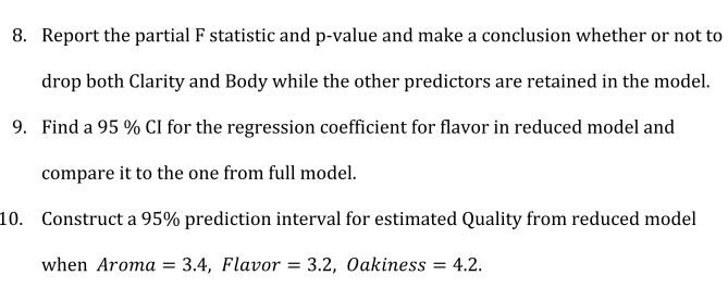
Q.7

Equation for reduced model,

quality = 6.4672 + 0.5801 Aroma + 1.1997 flavor - 0.6023 oakiness

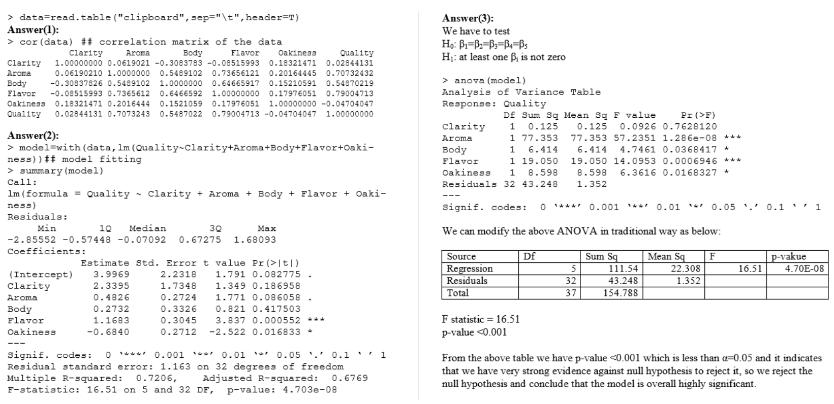
Answer(3): We have to test HO: Bi=B2=B3=B4=Bs Hj: at least one i is not zero > data=read.table ("clipboard", sep="\t", header=T) Answer(1): > cor (data) ## correlation matrix of the data Clarity Aroma Body Flavor Oakiness Quality Clarity 1.00000000 0.0619021 -0.3083783 -0.08515993 0.18321471 0.02844131 Aroma 0.06190210 1.0000000 0.5489102 0.73656121 0.20164445 0.70732432 Body -0.30837826 0.5489102 1.0000000 0.64665917 0.15210591 0.54870219 Flavor -0.08515993 0.7365612 0.6466592 1.00000000 0.17976051 0.79004713 Oakiness 0.18321471 0.2016444 0.1521059 0.17976051 1.00000000 -0.04704047 Quality 0.02844131 0.7073243 0.5487022 0.79004713 -0.04704047 1.00000000 > anova (model) Analysis of Variance Table Response: Quality DE Sum Sq Mean Sq F value Pr(>F) clarity 1 0.125 0.125 0.0926 0.7628120 Aroma 1 77.353 77.353 57.2351 1.286e-08 *** Body 1 6.414 6.414 4.7461 0.0368417 Flavor 1 19.050 19.050 14.0953 0.0006946 *** Oakiness 1 8.598 8.598 6.3616 0.0168327 Residuals 32 43.248 1.352 --- Signif. codes: O *** 0.001 **' 0.01 * 0.05 '.' 0.1'' 1 Answer(2): > model=with (data, lm (Quality-Clarity+Aroma+Body+Flavor+Oaki- ness)) ## model fitting > summary (model) Call: lm (formula = Quality clarity + Aroma + Body + Flavor + Oaki- ness) Residuals: Min 10 Median 30 Max -2.85552 -0.57448 -0.07092 0.67275 1.68093 Coefficients: Estimate Std. Error t value Pr (>tl) (Intercept) 3.9969 2.2318 1.791 0.082775 clarity 2.3395 1.7348 1.349 0.186958 Aroma 0.4826 0.2724 1.771 0.08 6058 Body 0.2732 0.3326 0.821 0.417503 Flavor 1.1683 0.3045 3.837 0.000552 Oakiness -0.6840 0.2712 -2.522 0.016833 We can modify the above ANOVA in traditional way as below: Df F Source Regression Residuals Total p-vakue 4.70E-08 16.51 Sum Sa 111.54 43.248 154.788 Mean Sq 22.308 1.352 5 32 37 F statistic = 16.51 p-value data=read.table ("clipboard", sep="\t", header=T) Answer(1): > cor (data) ## correlation matrix of the data Clarity Aroma Body Flavor Oakiness Quality Clarity 1.00000000 0.0619021 -0.3083783 -0.08515993 0.18321471 0.02844131 Aroma 0.06190210 1.0000000 0.5489102 0.73656121 0.20164445 0.70732432 Body -0.30837826 0.5489102 1.0000000 0.64665917 0.15210591 0.54870219 Flavor -0.08515993 0.7365612 0.6466592 1.00000000 0.17976051 0.79004713 Oakiness 0.18321471 0.2016444 0.1521059 0.17976051 1.00000000 -0.04704047 Quality 0.02844131 0.7073243 0.5487022 0.79004713 -0.04704047 1.00000000 > anova (model) Analysis of Variance Table Response: Quality DE Sum Sq Mean Sq F value Pr(>F) clarity 1 0.125 0.125 0.0926 0.7628120 Aroma 1 77.353 77.353 57.2351 1.286e-08 *** Body 1 6.414 6.414 4.7461 0.0368417 Flavor 1 19.050 19.050 14.0953 0.0006946 *** Oakiness 1 8.598 8.598 6.3616 0.0168327 Residuals 32 43.248 1.352 --- Signif. codes: O *** 0.001 **' 0.01 * 0.05 '.' 0.1'' 1 Answer(2): > model=with (data, lm (Quality-Clarity+Aroma+Body+Flavor+Oaki- ness)) ## model fitting > summary (model) Call: lm (formula = Quality clarity + Aroma + Body + Flavor + Oaki- ness) Residuals: Min 10 Median 30 Max -2.85552 -0.57448 -0.07092 0.67275 1.68093 Coefficients: Estimate Std. Error t value Pr (>tl) (Intercept) 3.9969 2.2318 1.791 0.082775 clarity 2.3395 1.7348 1.349 0.186958 Aroma 0.4826 0.2724 1.771 0.08 6058 Body 0.2732 0.3326 0.821 0.417503 Flavor 1.1683 0.3045 3.837 0.000552 Oakiness -0.6840 0.2712 -2.522 0.016833 We can modify the above ANOVA in traditional way as below: Df F Source Regression Residuals Total p-vakue 4.70E-08 16.51 Sum Sa 111.54 43.248 154.788 Mean Sq 22.308 1.352 5 32 37 F statistic = 16.51 p-value