Use the data provided in the case study to tabulate the cashflows of the interest rate swap based on the two rates and the value of the corresponding swap? Show all calculations in detail and report the method or equation used in undertaking calculations.Explain the similarity or differences in value according to valuation.

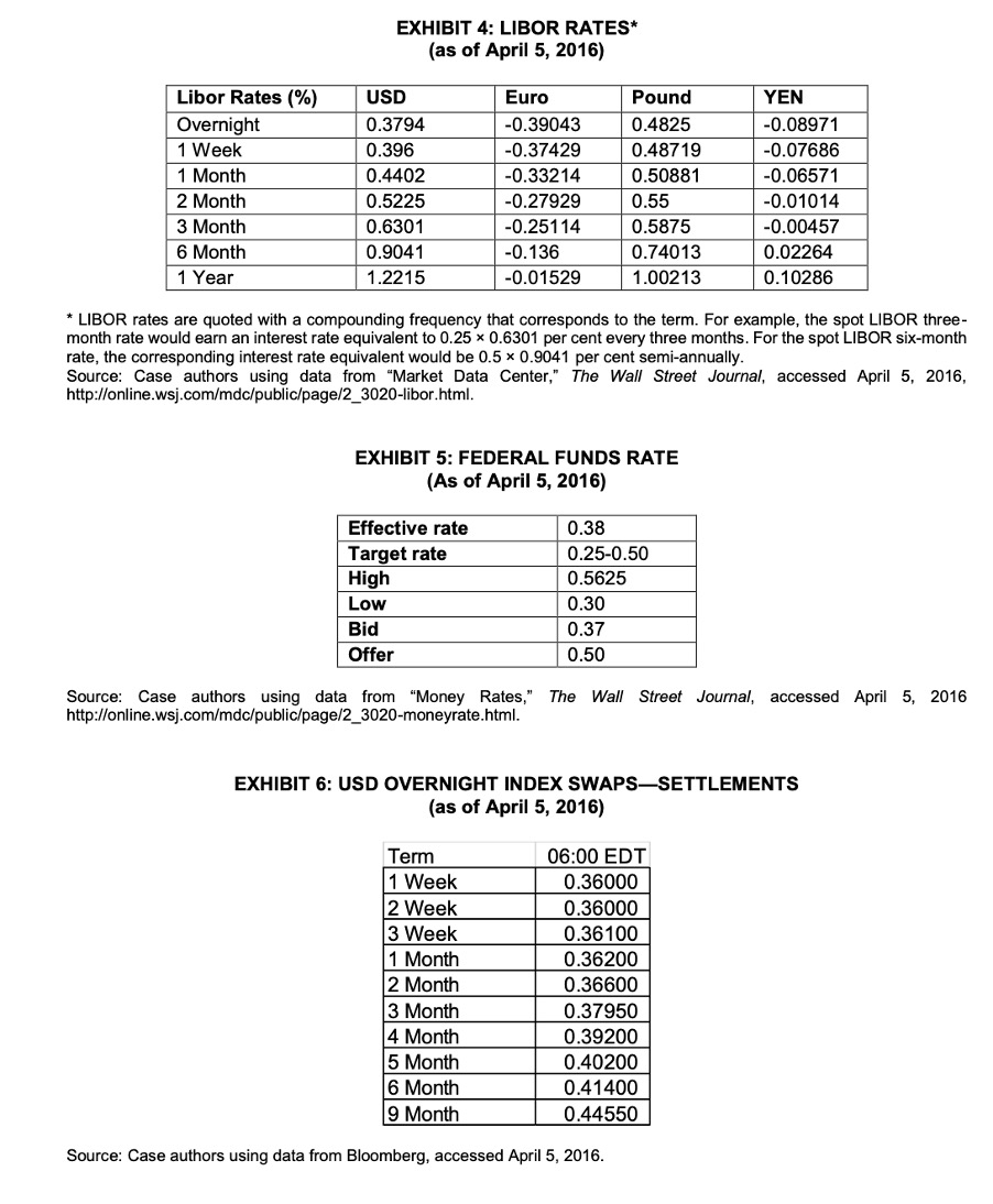
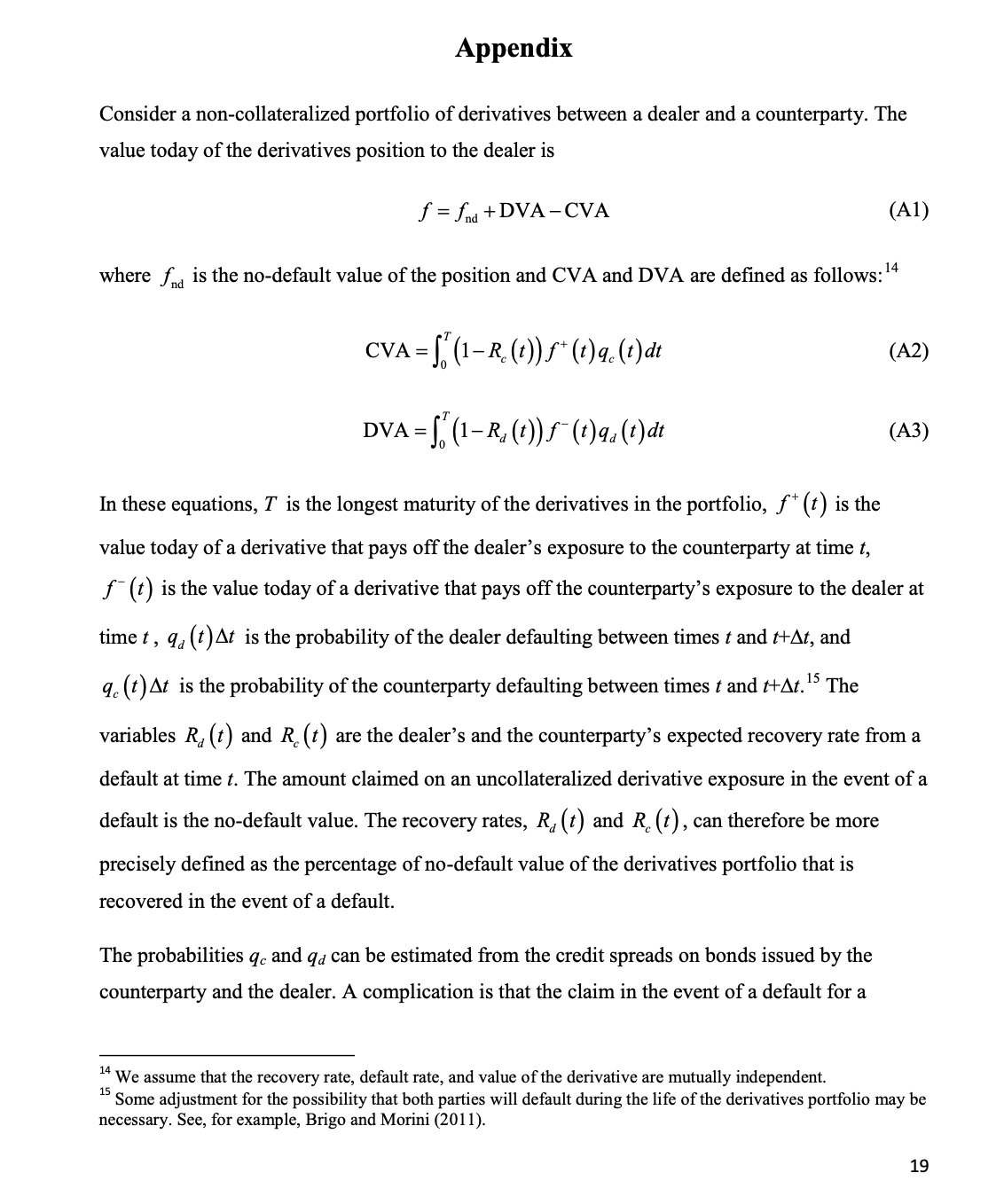
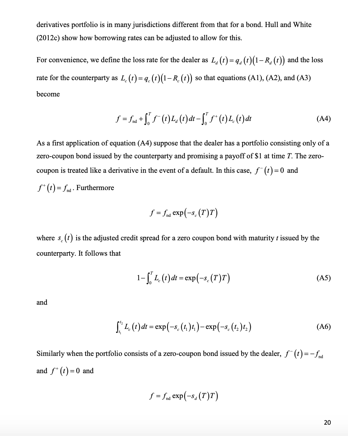
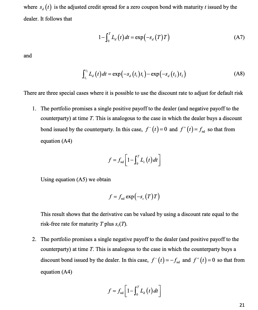
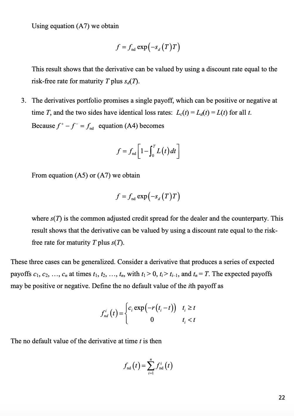
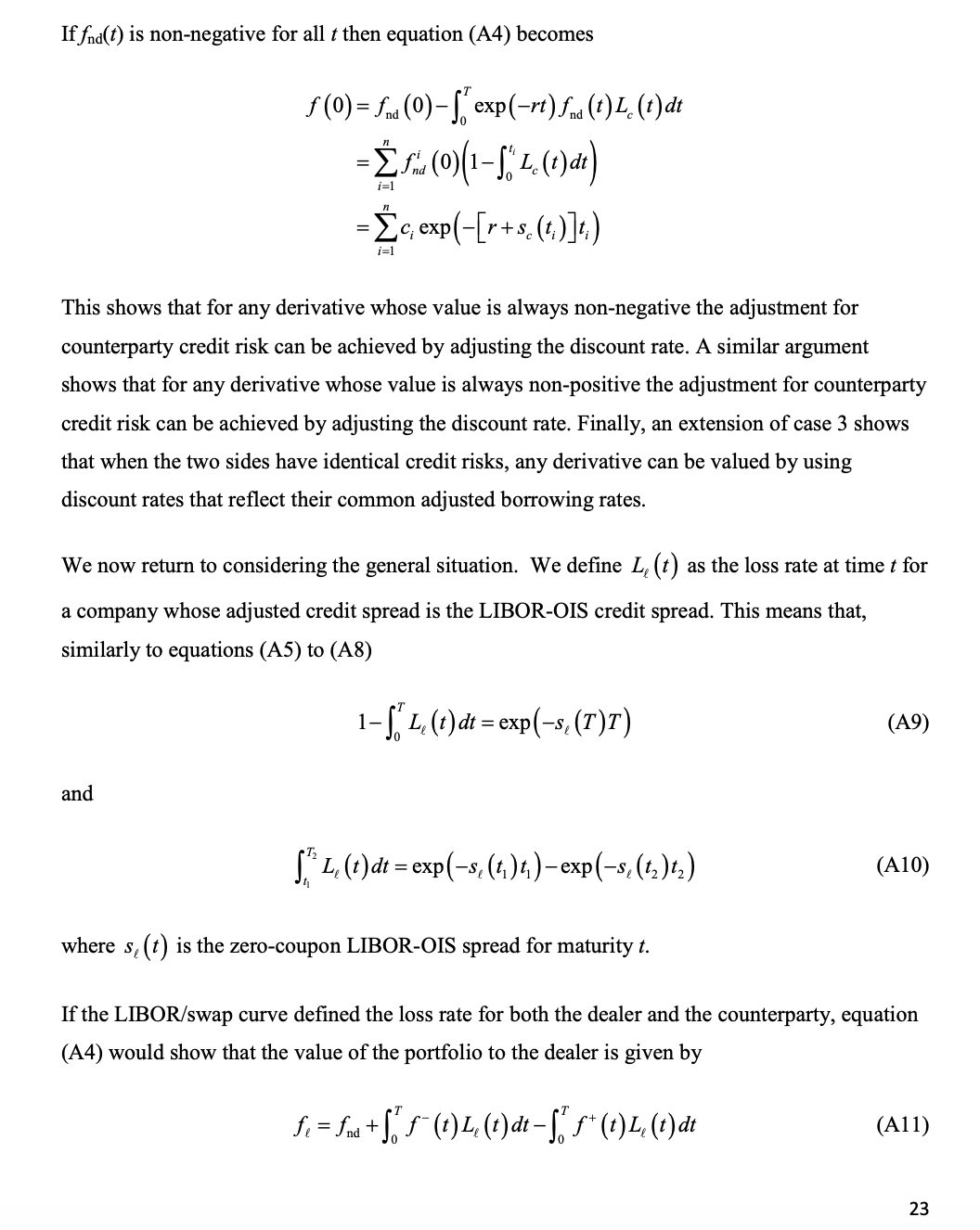
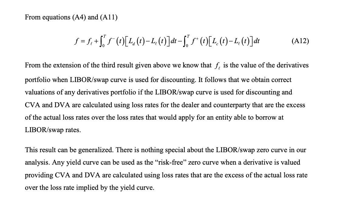
EXHIBIT 4: LIBOR RATES* (as of April 5, 2016) Libor Rates (%) USD Euro Pound YEN Overnight 0.3794 -0.39043 0.4825 -0.08971 1 Week 0.396 -0.37429 0.48719 -0.07686 1 Month 0.4402 -0.33214 0.50881 0.06571 2 Month 0.5225 -0.27929 0.55 -0.01014 3 Month 0.6301 -0.25114 0.5875 -0.00457 6 Month 0.9041 -0.136 0.74013 0.02264 1 Year 1.2215 -0.01529 1.00213 0.10286 * LIBOR rates are quoted with a compounding frequency that corresponds to the term. For example, the spot LIBOR three- month rate would earn an interest rate equivalent to 0.25 x 0.6301 per cent every three months. For the spot LIBOR six-month ate, the corresponding interest rate equivalent would be 0.5 x 0.9041 per cent semi-annually. Source: Case authors using data from "Market Data Center," The Wall Street Journal, accessed April 5, 2016, http://online.wsj.com/mdc/public/page/2_3020-libor.html. EXHIBIT 5: FEDERAL FUNDS RATE (As of April 5, 2016) Effective rate 0.38 Target rate 0.25-0.50 High 0.5625 Low 0.30 Bid 0.37 Offer 0.50 Source: Case authors using data from "Money Rates," The Wall Street Journal, accessed April 5, 2016 http://online.wsj.com/mdc/public/page/2_3020-moneyrate.html. EXHIBIT 6: USD OVERNIGHT INDEX SWAPS-SETTLEMENTS (as of April 5, 2016) Term 06:00 EDT 1 Week 0.36000 2 Week 0.36000 3 Week 0.36100 1 Month 0.36200 2 Month 0.36600 3 Month 0.37950 4 Month 0.39200 5 Month 0.40200 6 Month 0.41400 9 Month 0.44550 Source: Case authors using data from Bloomberg, accessed April 5, 2016.Appendix Consider a non-collateralized portfolio of derivatives between a dealer and a counterparty. The value today of the derivatives position to the dealer is f = find + DVA-CVA (Al) where find is the no-default value of the position and CVA and DVA are defined as follows: CVA =[ (1-R. (t)) f+ (t) q. (t) at (A2) DVA =[. (1-R. (t)) f (t) qa (t) at (A3) In these equations, T is the longest maturity of the derivatives in the portfolio, f+ (t) is the value today of a derivative that pays off the dealer's exposure to the counterparty at time t, f (t) is the value today of a derivative that pays off the counterparty's exposure to the dealer at time t, qa (t) At is the probability of the dealer defaulting between times t and t+At, and de (t) At is the probability of the counterparty defaulting between times t and t+At." The variables Ra (t) and R. (t) are the dealer's and the counterparty's expected recovery rate from a default at time t. The amount claimed on an uncollateralized derivative exposure in the event of a default is the no-default value. The recovery rates, Ra (t) and R. (t) , can therefore be more precisely defined as the percentage of no-default value of the derivatives portfolio that is recovered in the event of a default. The probabilities qe and qa can be estimated from the credit spreads on bonds issued by the counterparty and the dealer. A complication is that the claim in the event of a default for a We assume that the recovery rate, default rate, and value of the derivative are mutually independent. Some adjustment for the possibility that both parties will default during the life of the derivatives portfolio may be necessary. See, for example, Brigo and Morini (2011). 19derivatives portfolio is in many jurisdictions different from that for a bond. Hull and White (2012c) show how borrowing rates can be adjusted to allow for this. For convenience, we define the loss rate for the dealer as La (t) = qa (t) (1-Ra (t)) and the loss rate for the counterparty as L. (t) = q. (t) (1-R. (t)) so that equations (Al), (A2), and (A3) become f = fnd + 1. f- (t ) I. (1 ) at - 1 " f* ( t ) I . (1 ) at (A4) As a first application of equation (A4) suppose that the dealer has a portfolio consisting only of a zero-coupon bond issued by the counterparty and promising a payoff of $1 at time T. The zero- coupon is treated like a derivative in the event of a default. In this case, f (t) =0 and f* (t) = fnd. Furthermore f = find exp(-s. (T)T) where s. (t) is the adjusted credit spread for a zero coupon bond with maturity t issued by the counterparty. It follows that 1-J. L. (1) dt = exp(-s. (I)I) (A5) and [" L. (t) dt = exp(-s.(1,)1)-exp(-s. (12) $2) (A6) Similarly when the portfolio consists of a zero-coupon bond issued by the dealer, f (t) = -fnd and f* (t) =0 and f = fnd exp(-sa (T) T) 20where sd (t) is the adjusted credit spread for a zero coupon bond with maturity it issued by the dealer. It follows that 141"ch (t)dt = exp(Sa. my") (A?) 0 and I: La, (ak = exp (sd (t1 )t1 ) exp(.s-d (12):?!) (A8) There are three special cases where it is possible to use the discount rate to adjust for default risk 1. The portfolio promises a single positive payoff to the dealer (and negative payoff to the counterparty) at time T. This is analogous to the case in which the dealer buys a discount bond issued by the counterparty. In this case, f ' (t) = 0 and f + (t) = f\"11d so that from equation (A4) f: fm [1136 (r)dt] 0 Using equatiOn (AS) we obtain 1\" = fad exp(sc (T)T) This result shows that the derivative can be valued by using a discount rate equal to the risk-free rate for maturity T plus 56(7). 2. The portfolio promises a single negative payoff to the dealer (and positive payoff to the counterparty) at time T. This is analogous to the case in which the counterparty buys a discount bond issued by the dealer. In this case, f' (I) = m and f (t) = 0 so that from equatiOn (A4) T f=fnd[1j'0 Ld(t)dt:| 21 Using equatirm (A?) we obtain f =fnd exp(sd (T)T) This result shows that the derivative can be valued by using a discount rate equal to the risk-free rate for maturity T plus 3.;(7'). . The derivatives portfolio promises a single payoff, which can be positive or negative at time T, and the two sides have identical loss rates: L130) = Lara) = L(r) for all r. Because 1\" f' = m equatiOn (A4) becomes f = 3d [1IOTL(:)dz] From equation (A5) or (A?) we obtain f =fmi exp(sd (T)T) where 3(7) is the commOn adjusted credit spread for the dealer and the counterparty. This result shows that the derivative can be valued by using a discount rate equal to the risk- ee rate for maturity T plus 3(1). These three cases can be generalized. Consider a derivative that produces a series of expected payoffs 01, C2, ..., c" at times :1, t2, ..., tn, with 31> 0, t; > n.1, and a, = T. The expected payoffs may be positive or negative. Dene the no default value of the ith payoff as f; (t) ={C' exP(_r('r' \"D r.- 2 r 0 no: The no default value of the derivative at time t is then novice) i=1 22 If fna(t) is non-negative for all t then equation (A4) becomes f (0) = And ( 0) -[ exp (-rt) find (t ) L. (t) dt =[ fid (0) ( 1-[" L. (t) at -Eq,exp(-[r+s. (1,) ]t.) This shows that for any derivative whose value is always non-negative the adjustment for counterparty credit risk can be achieved by adjusting the discount rate. A similar argument shows that for any derivative whose value is always non-positive the adjustment for counterparty credit risk can be achieved by adjusting the discount rate. Finally, an extension of case 3 shows that when the two sides have identical credit risks, any derivative can be valued by using discount rates that reflect their common adjusted borrowing rates. We now return to considering the general situation. We define Le (t ) as the loss rate at time t for a company whose adjusted credit spread is the LIBOR-OIS credit spread. This means that, similarly to equations (A5) to (A8) 1-J. L, (t) dt = exp(-s, (T) I) (A9) and [." L, (1 ) dt = exp(-s, (1,)1)-exp(-s,(12) tz) (A10) where s, (t) is the zero-coupon LIBOR-OIS spread for maturity t. If the LIBOR/swap curve defined the loss rate for both the dealer and the counterparty, equation (A4) would show that the value of the portfolio to the dealer is given by fe = fod + S. f- ( t ) I, ( 1 ) at - 15 5+ ( t ) I, (1 ) at (All) 23From equations (A4) and (A1 1) f = )3 +jon' (t)[Ld (t)L (z)]dtj:f+ (t)[Lc (z)L,_. (t)]dt (A12) From the extension of the third result given above we know that 1:, is the value of the derivatives portfolio when LIBORJ'swap curve is used for discounting. It follows that we obtain correct valuations of any derivatives portfolio if the LIBORfswap curve is used for discounting and CVA and DVA are calculated using loss rates for the dealer and counterparty that are the excess of the actual loss rates over the loss rates that would apply for an entity able to borrow at LIBORfswap rates. This result can be generalized. There is nothing special about the LIBOR/swap zero curve in our analysis. Any yield curve can be used as the \"risk-free\" zero curve when a derivative is valued providing CVA and DVA are calculated using loss rates that are the excess of the actual loss rate over the loss rate implied by the yield curve