use the sample code to answer 3&4

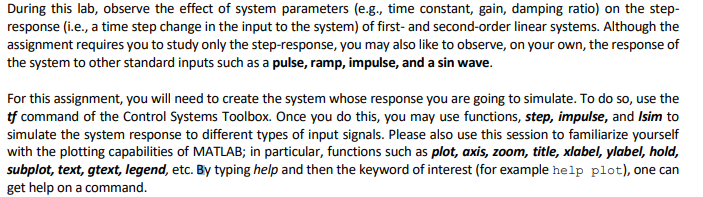
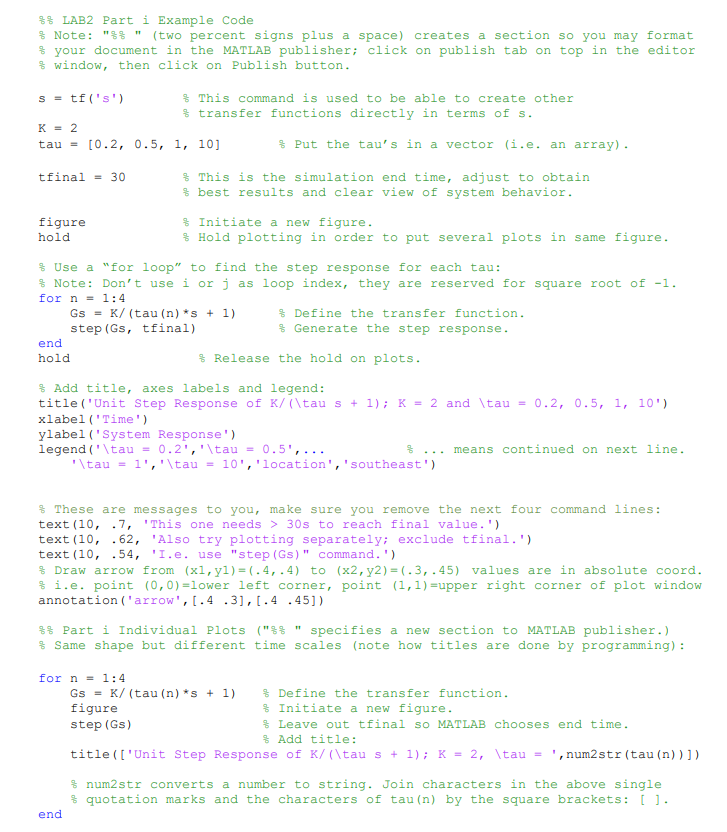
During this lab, observe the effect of system parameters (e.g., time constant, gain, damping ratio) on the step- response (i.e., a time step change in the input to the system) of first- and second-order linear systems. Although the assignment requires you to study only the step-response, you may also like to observe, on your own, the response of the system to other standard inputs such as a pulse, ramp, impulse, and a sin wave. For this assignment, you will need to create the system whose response you are going to simulate. To do so, use the tf command of the Control Systems Toolbox. Once you do this, you may use functions, step, impulse, and Isim to simulate the system response to different types of input signals. Please also use this session to familiarize yourself with the plotting capabilities of MATLAB; in particular, functions such as plot, axis, zoom, title, xlabel, ylabel, hold, subplot, text, gtext, legend, etc. By typing help and then the keyword of interest (for example help plot), one can get help on a command. $$ LAB2 Part i Example Code $ Note: "" (two percent signs plus a space) creates a section so you may format $ your document in the MATLAB Publisher; click on publish tab on top in the editor $ window, then click on Publish button. s = tf('s') $ This command is used to be able to create other % transfer functions directly in terms of s. K = 2 tau = [0.2, 0.5, 1, 10] % Put the tau's in a vector (i.e. an array). tfinal = 30 $ This is the simulation end time, adjust to obtain % best results and clear view of system behavior. $ Initiate a new figure. $ Hold plotting in order to put several plots in same figure. figure hold % Use a "for loop" to find the step response for each tau: $ Note: Don't use i orj as loop index, they are reserved for square root of -1. for n = 1:4 Gs = K/ (tau (n)*5 + 1) Define the transfer function. step (Gs, tfinal) $ Generate the step response. end hold $ Release the hold on plots. % Add title, axes labels and legend: title('Unit Step Response of K/(\tau s + 1); K = 2 and \tau = 0.2, 0.5, 1, 10') xlabel('Time') ylabel('System Response') legend('\tau = 0.2','\tau = 0.5',... means continued on next line. \tau = l','\tau = 10', 'location','southeast') These are messages to you, make sure you remove the next four command lines: text (10, .7, 'This one needs > 30s to reach final value.') text (10, .62, 'Also try plotting separately; exclude tfinal.') text (10, .54, 'I.e. use "step (Gs)" command.') % Draw arrow from (x1, y1)=(-4, .4) to (x2, y2) = (-3, .45) values are in absolute coord. fi.e. point (0,0) =lower left corner, point (1,1)=upper right corner of plot window annotation ('arrow', 1.4.3],[.4 .45]) $$ Part i Individual Plots ("%% specifies a new section to MATLAB publisher.) % Same shape but different time scales (note how titles are done by programming): for n = 1:4 Gs = K/(tau (n) *s + 1) $ Define the transfer function. figure % Initiate a new figure. step (Gs) Leave out tfinal so MATLAB chooses end time. Add title: title(['Unit Step Response of K/(\tau s + 1); K = 2, \tau = ', num2str (tau (n))]) $ num2str converts a number to string. Join characters in the above single $ quotation marks and the characters of tau (n) by the square brackets: []. end During this lab, observe the effect of system parameters (e.g., time constant, gain, damping ratio) on the step- response (i.e., a time step change in the input to the system) of first- and second-order linear systems. Although the assignment requires you to study only the step-response, you may also like to observe, on your own, the response of the system to other standard inputs such as a pulse, ramp, impulse, and a sin wave. For this assignment, you will need to create the system whose response you are going to simulate. To do so, use the tf command of the Control Systems Toolbox. Once you do this, you may use functions, step, impulse, and Isim to simulate the system response to different types of input signals. Please also use this session to familiarize yourself with the plotting capabilities of MATLAB; in particular, functions such as plot, axis, zoom, title, xlabel, ylabel, hold, subplot, text, gtext, legend, etc. By typing help and then the keyword of interest (for example help plot), one can get help on a command. $$ LAB2 Part i Example Code $ Note: "" (two percent signs plus a space) creates a section so you may format $ your document in the MATLAB Publisher; click on publish tab on top in the editor $ window, then click on Publish button. s = tf('s') $ This command is used to be able to create other % transfer functions directly in terms of s. K = 2 tau = [0.2, 0.5, 1, 10] % Put the tau's in a vector (i.e. an array). tfinal = 30 $ This is the simulation end time, adjust to obtain % best results and clear view of system behavior. $ Initiate a new figure. $ Hold plotting in order to put several plots in same figure. figure hold % Use a "for loop" to find the step response for each tau: $ Note: Don't use i orj as loop index, they are reserved for square root of -1. for n = 1:4 Gs = K/ (tau (n)*5 + 1) Define the transfer function. step (Gs, tfinal) $ Generate the step response. end hold $ Release the hold on plots. % Add title, axes labels and legend: title('Unit Step Response of K/(\tau s + 1); K = 2 and \tau = 0.2, 0.5, 1, 10') xlabel('Time') ylabel('System Response') legend('\tau = 0.2','\tau = 0.5',... means continued on next line. \tau = l','\tau = 10', 'location','southeast') These are messages to you, make sure you remove the next four command lines: text (10, .7, 'This one needs > 30s to reach final value.') text (10, .62, 'Also try plotting separately; exclude tfinal.') text (10, .54, 'I.e. use "step (Gs)" command.') % Draw arrow from (x1, y1)=(-4, .4) to (x2, y2) = (-3, .45) values are in absolute coord. fi.e. point (0,0) =lower left corner, point (1,1)=upper right corner of plot window annotation ('arrow', 1.4.3],[.4 .45]) $$ Part i Individual Plots ("%% specifies a new section to MATLAB publisher.) % Same shape but different time scales (note how titles are done by programming): for n = 1:4 Gs = K/(tau (n) *s + 1) $ Define the transfer function. figure % Initiate a new figure. step (Gs) Leave out tfinal so MATLAB chooses end time. Add title: title(['Unit Step Response of K/(\tau s + 1); K = 2, \tau = ', num2str (tau (n))]) $ num2str converts a number to string. Join characters in the above single $ quotation marks and the characters of tau (n) by the square brackets: []. end