Using Python to have q plot of a graph

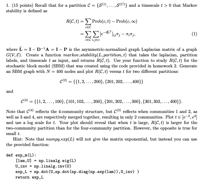
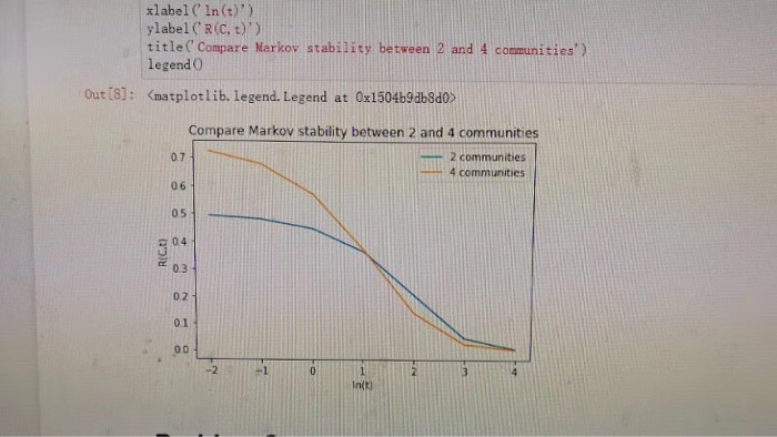
1. (15 points) Recall that for a partition C SSC)y and a timescale t > 0 that Markov stability is defined as R(C,t)-Prob(c,t) -Prob(e, oo) CEC where L = 1-D-A-1-P is the asymmetric-normalized graph Laplacian matrix of a graph GV,E). Create a function markov-stability(L, partition, t) that takes the laplacian, partition labels, and timescale t as input, and returns R(C, t). Use your function to study R(C, t) for the stochastic block model (SBM) that was created using the code provided in homework 2. Generate an SBM graph with N-400 nodes and plot R(C, t) versus t for two different partitions c(2)-1,2,...,200), (201, 202,... ,400)) an e = {{1, 2, . . . , 100}, { 101, 102, . . . , 200), {201, 202, . . . , 300), {301, 302, . . . ,400)) Note that C(4) reflects the 4-community structure, but C(2) reflects when communities 1 and 2, as well as 3 and 4, are respectively merged together, resulting in only 2 communities. Plot tE e-2,e4] and use a log scale for t. Your plot should reveal that when t is large, R(C, t) is larger for the two-community partition than for the four-community partition. However, the opposite is true for small t Hint: Note that numpy.exp(L) will not give the matrix exponential, but instead you can use the provided function: def exp_m (L) [1am , U] = np. linalg. eig(L) U_inv - np.linalg.inv (U) exp-L = np. dot (U , np. dot (np. diag (np. exp (1am)),U-inv) return exp_L ) xlabel( In (t)') ylabel(R(C, D)) title( Compare Markov stability between 2 and 4 communities') legend 0 Out (6]: Kmatplotlib. legend. Legend at ox1504b9ab8do Compare Markov stability between 2 and 4 communities 2 communities 4 communities 0.7 0.6 05 C 04 0.3 0.2 01 ,004 -2 In(t) 1. (15 points) Recall that for a partition C SSC)y and a timescale t > 0 that Markov stability is defined as R(C,t)-Prob(c,t) -Prob(e, oo) CEC where L = 1-D-A-1-P is the asymmetric-normalized graph Laplacian matrix of a graph GV,E). Create a function markov-stability(L, partition, t) that takes the laplacian, partition labels, and timescale t as input, and returns R(C, t). Use your function to study R(C, t) for the stochastic block model (SBM) that was created using the code provided in homework 2. Generate an SBM graph with N-400 nodes and plot R(C, t) versus t for two different partitions c(2)-1,2,...,200), (201, 202,... ,400)) an e = {{1, 2, . . . , 100}, { 101, 102, . . . , 200), {201, 202, . . . , 300), {301, 302, . . . ,400)) Note that C(4) reflects the 4-community structure, but C(2) reflects when communities 1 and 2, as well as 3 and 4, are respectively merged together, resulting in only 2 communities. Plot tE e-2,e4] and use a log scale for t. Your plot should reveal that when t is large, R(C, t) is larger for the two-community partition than for the four-community partition. However, the opposite is true for small t Hint: Note that numpy.exp(L) will not give the matrix exponential, but instead you can use the provided function: def exp_m (L) [1am , U] = np. linalg. eig(L) U_inv - np.linalg.inv (U) exp-L = np. dot (U , np. dot (np. diag (np. exp (1am)),U-inv) return exp_L ) xlabel( In (t)') ylabel(R(C, D)) title( Compare Markov stability between 2 and 4 communities') legend 0 Out (6]: Kmatplotlib. legend. Legend at ox1504b9ab8do Compare Markov stability between 2 and 4 communities 2 communities 4 communities 0.7 0.6 05 C 04 0.3 0.2 01 ,004 -2 In(t)