

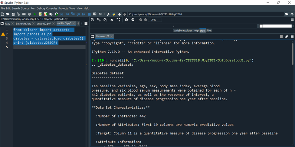
Question: Using the Scikit-Learn Dataset To load the sample scikit data set, import the datasets module and load the desired dataset. Code Run: from sklearn import
Using the Scikit-Learn Dataset
To load the sample scikit data set, import the datasets module and load the desired dataset.
Code Run:
from sklearn import datasets
import pandas as pd
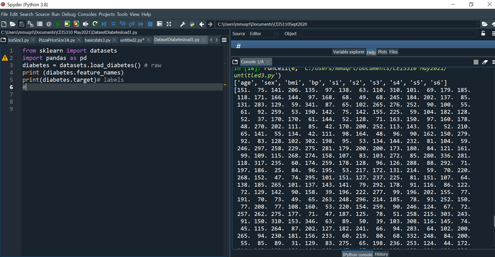
diabetes = datasets.load_diabetes() # raw
print (diabetes.DESCR)
Besides the diabetes dataset, one can also load some other interesting datasets in Scikit-learn such as the following.
breast_cancer = datasets.load_breast_cancer( ) # data on breast cancer
The print(feature-names) property of the dataset prints the names of the dataset features.
Activity I:
- Open any of your favorite Python IDE.
- Also run the given code snippet for digits dataset of 1797 8 x 8 images of hand-written digits.
- Using the three different print statements to explore each:features, feature_names and target_names properties and enclose screenshot of your outputs for each of the properties for digits.
- Modify the code snippet given above to access Iris Flower data from your ScikitLearn library.
- Use Python commands to explore the Iris Data set and enclose your findings.
from sklearn import datasets
import pandas as pd
digits = datasets.load_digits()
print(digits.target_names)
print(digits.feature_names)
df = pd.DataFrame(digits.data)
print(df.head())
Generating Your Own Dataset
You can generate yourself a suitable data set for your machine learning experimentation.
You can use the sklearn.datasets.samples_generator module from the Scikit-learn library (which contains a number of functions) to let you generate different types of datasets for different types of problems.
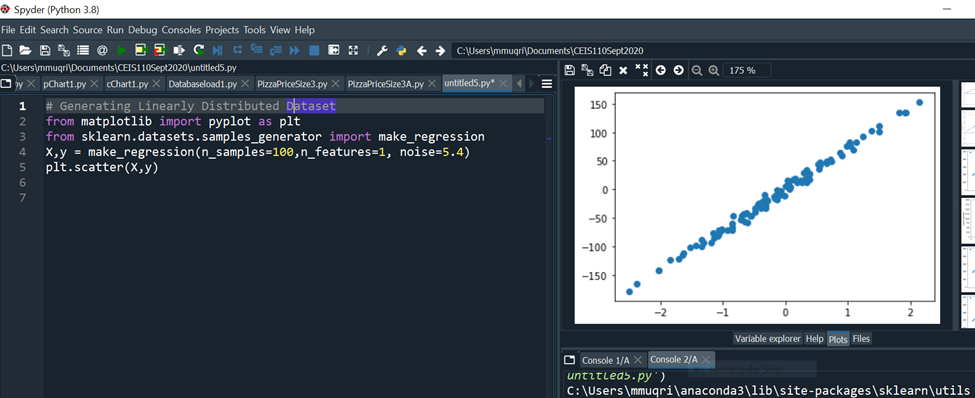
Linearly Distributed Dataset
The make_regression() function generates linearly distributed data points, allows you to specify the desired number of features and the standard deviation of the Gaussian noise applied to the output.
Code run: # Generating Linearly Distributed Dataset
from matplotlib import pyplot as plt
from sklearn.datasets.samples_generator import make_regression
X,y = make_regression(n_samples=100,n_features=1, noise=5.4)
plt.scatter(X,y)
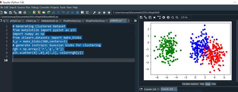
Clustered Dataset
The make_blobs() function generates n number of clusters of random data. This is quite useful when performing clustering in unsupervised learning, as well as in Supervised Learning- Classification using K Nearest Neighbors(KNN).
Code Run: # Generating Clustered Dataset
from matplotlib import pyplot as plt
import numpy as np
from sklearn.datasets import make_blobs
X,y = make_blobs(500,centers=3)
# generate isotropic Gaussian blobs for clustering
rgb = np.array(['r','g','b'])
plt.scatter(X[:,0],X[:,1], color=rgb[y])
The figure below shows the scatter plot of the random generated dataset.
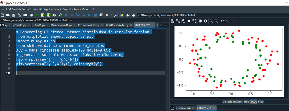
Clustered Dataset Distributed in Circular Fashion
The make_circles() function generates a random data set containing a large circle embedding a smaller circle in two dimensions. This is useful when performing classifications, using algorithms such as SVM (Support Vector Machines).
Code Run: # Generating Clustered Dataset Distributed in Circular Fashion
# Generating Clustered Dataset distributed in circular fashion
from matplotlib import pyplot as plt
import numpy as np
from sklearn.datasets import make_circles
X,y = make_circles(n_samples=100,noise=0.09)
rgb = np.array(['r','g','b'])
plt.scatter(X[:,0],X[:,1], color=rgb[y])
- Include a screenshot from Windows Explorer showing the dataset you explored
- Include a screenshot from Spyder showing your Python code and screen output for Activity 1 with your name and date in the comments.
*Include a screenshot from Spyder showing your Python code and screen output for Activity 2with your name and date in the comments
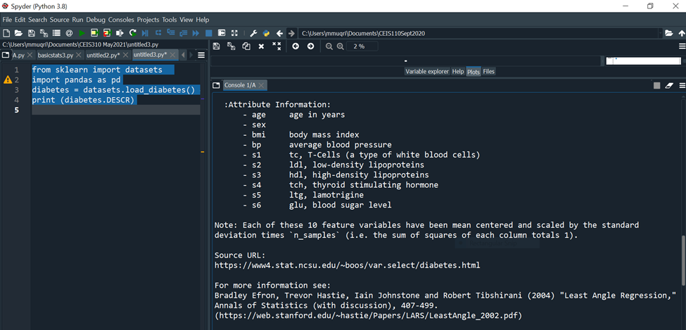
C:YUsersimmuqri|Documents|CEIS110Sept2020 Variable explorer Help Plots Files Console 1/A Type "copyright", "credits" or "license" for more information. IPython 7.19 .0 -- An enhanced Interactive Python. In [10]: runcell(0, 'C:/Users/mmuqri/Documents/CEIS310 May2021/Databaseload1.py') . _diabetes_dataset: Diabetes dataset Ten baseline variables, age, sex, body mass index, average blood pressure, and six blood serum measurements were obtained for each of n= 442 diabetes patients, as well as the response of interest, a quantitative measure of disease progression one year after baseline. **Data Set Characteristics:** :Number of Instances: 442 :Number of Attributes: First 10 columns are numeric predictive values :Target: Column 11 is a quantitative measure of disease progression one year after baseline :Attribute Information: C:V)(Users/mmugri) Documents/CEIS110Sept2020 Varlable explorer Help Plots files Console 1/A :Attribute Information: - age age in years - sex - bmi body mass index - bp average blood pressure - s1 tc, T-Cells (a type of white blood cells) - s2 ldl, low-density lipoproteins - s3 hdl, high-density lipoproteins - s4 tch, thyroid stimulating hormone - s5 ltg, lamotrigine - s6 glu, blood sugar level Note: Each of these 10 feature variables have been mean centered and scaled by the standard deviation times "n_samples" (i.e. the sum of squares of each column totals 1). Source URL: https://www4.stat.ncsu.edu/ boos/var.select/diabetes.html For more information see: Bradley Efron, Trevor Hastie, Iain Johnstone and Robert Tibshirani (2004) "Least Angle Regression," Annals of Statistics (with discussion), 407-499. (https://web.stanford.edu/ whastie/Papers/LARS/LeastAngle_2002.pdf) Spyder (Python 3.8) File Edit Search Source Run Debug Consoles Projects Tools View Help (i) C c C:Users/mmuqri|Documents/CEIS110Sept2020 C: (Users/mmuqri|Documents/CEIS310 May20211DatasetDlabetesload1.py icesize3.p Pimapicesize3A.py basictats3.py untitled2.py* DatasetDiabetesload1.py 1 42 3 4 5 6 7 8 9 from sklearn import datasets import pandas as pd diabetes = datasets.load_diabetes () \# raw print (diabetes.feature_names) print(diabetes.target)\# labels Source Editor Object \# Variable explorer Help Plots files Console 1/A [20] untitled3.py') ['age', 'sex', 'bmi', 'bp', 's1', 's2', 's3', 's4', 's5', 's6'] [151. 75. 141. 206. 135. 97. 138. 63. 110. 310. 101. 69. 179. 185. 118. 171. 166. 144. 97. 168. 68. 49. 68. 245. 184. 202. 137. 85. 131. 283. 129. 59. 341.87,65,102,265,276,252.90,100.55. 61. 92. 259. 53. 190. 142. 75. 142. 155. 225. 59. 104. 182. 128. 52. 37. 170.170 .61 .144 .52 .128 .71 .163 .150 .97 .160 .178 \). 48. 270.202 . 111. 85. 42. 170. 200. 252. 113. 143. 51. 52. 210. 65. 141. 55. 134. 42. 111. 98. 164. 48. 96. 90. 162. 150. 279. 92. 83. 128. 102. 302. 198. 95. 53. 134. 144. 232. 81. 104. 59. 246. 297. 258. 229. 275. 281. 179. 200. 200. 173. 180. 84. 121. 161. 99. 109. 115. 268. 274. 158. 107. 83. 103. 272. 85. 280. 336. 281. 118. 317.235.60.174.259.178,128.96.126.288.88.292.71. 197. 186. 25. 84. 96. 195. 53. 217. 172. 131. 214. 59. 70. 220. 268. 152. 47. 74. 295. 101. 151. 127. 237. 225. 81. 151. 107. 64. 138. 185. 265. 101. 137. 143. 141. 79. 292. 178. 91. 116. 86. 122. 72. 129. 142. 90. 158. 39. 196. 222. 277. 99. 196. 202. 155.77. 191. 70. 73. 49. 65.263 .248 .296 .214 .185 .78 .93 .252 .150 \). 77. 208. 77. 108. 160. 53. 220. 154. 259. 90. 246. 124. 67. 72. 257. 262. 275. 177. 71. 47. 187. 125. 78. 51. 258. 215. 303. 243. 91. 150. 310. 153. 346. 63. 89. 50. 39. 103. 308. 116. 145. 74. 45. 115. 264. 87. 202. 127. 182. 241. 66. 94. 283. 64. 102. 200. 265. 94. 230. 181. 156. 233. 60. 219. 80. 68. 332. 248. 84. 200. 55. 85. 89. 31. 129. 83. 275. 65. 198. 236. 253. 124. 44. 172. IPython console Hilstory \# Generating Linearly Distributed Dptaset from matplotlib import pyplot as plt from sklearn.datasets.samples_generator import make_regression x,y= make_regression(n_samples =100, n_features =1, noise =5.4 ) plt. scatter(X,y) Variable explorer Help Plots Files Console 1/A Console 2/A untrtleas.py ') C:\Users\mmuqri\anaconda3\lib\site-packages\sklearn\utils le Edit Search Source Run Debug Consoles Projects Tools View Help C:Usersimmuqri|Docume WUsers/mmuqri|Documents/CEIS110Sept2020/untitled5.py y pChart1.py cChart1.py Databaseload1.py PimaPriceSize3.py PimaPriceSize3A.py untitled5.py* \# Generating clustered Dataset from matplotlib import pyplot as plt import numpy as np from sklearn.datasets import make_blobs X,y= make_blobs (500, centers =3 ) \# generate isotropic Guassian blobs for clustering rgb=nparray([I,g,b]) plt.scatter(X[:,0],X[:,1], color=rgb[y]) ile Edit Search Source Run Debug Consoles Projects Tools View Help C:Users|mmuqriVocume :Users/mmuqri|Documents\CEIS110Sept2020/untitledS.py oy pChart1.py chart1.py Databaseload1.py PizzaPriceSize3.py PizaPriceSize3A.py untitled5.py* \[ \begin{array}{l} \text { \# Generating Clustered Dataset distributed in circular fashion } \\ \text { from matplotlib import pyplot as plt } \\ \text { import numpy as np } \\ \text { from sklearn.datasets import make_circles } \\ \mathrm{x}, \mathrm{y}=\text { make_circles (n_samples }=100 \text {, noise }=0.09 \text { ) } \\ \text { \# generate isotropic Guassian blobs for clustering } \\ r g b=n p . \operatorname{array}\left(\left[{ }^{\prime} r \text { ', ' } g{ }^{\prime}, ' b ' ight] ight) \\ \text { plt.scatter }(X[:, 0], X[:, 1], \operatorname{color}=r g b[y]) \\ \end{array} \] C:YUsersimmuqri|Documents|CEIS110Sept2020 Variable explorer Help Plots Files Console 1/A Type "copyright", "credits" or "license" for more information. IPython 7.19 .0 -- An enhanced Interactive Python. In [10]: runcell(0, 'C:/Users/mmuqri/Documents/CEIS310 May2021/Databaseload1.py') . _diabetes_dataset: Diabetes dataset Ten baseline variables, age, sex, body mass index, average blood pressure, and six blood serum measurements were obtained for each of n= 442 diabetes patients, as well as the response of interest, a quantitative measure of disease progression one year after baseline. **Data Set Characteristics:** :Number of Instances: 442 :Number of Attributes: First 10 columns are numeric predictive values :Target: Column 11 is a quantitative measure of disease progression one year after baseline :Attribute Information: C:V)(Users/mmugri) Documents/CEIS110Sept2020 Varlable explorer Help Plots files Console 1/A :Attribute Information: - age age in years - sex - bmi body mass index - bp average blood pressure - s1 tc, T-Cells (a type of white blood cells) - s2 ldl, low-density lipoproteins - s3 hdl, high-density lipoproteins - s4 tch, thyroid stimulating hormone - s5 ltg, lamotrigine - s6 glu, blood sugar level Note: Each of these 10 feature variables have been mean centered and scaled by the standard deviation times "n_samples" (i.e. the sum of squares of each column totals 1). Source URL: https://www4.stat.ncsu.edu/ boos/var.select/diabetes.html For more information see: Bradley Efron, Trevor Hastie, Iain Johnstone and Robert Tibshirani (2004) "Least Angle Regression," Annals of Statistics (with discussion), 407-499. (https://web.stanford.edu/ whastie/Papers/LARS/LeastAngle_2002.pdf) Spyder (Python 3.8) File Edit Search Source Run Debug Consoles Projects Tools View Help (i) C c C:Users/mmuqri|Documents/CEIS110Sept2020 C: (Users/mmuqri|Documents/CEIS310 May20211DatasetDlabetesload1.py icesize3.p Pimapicesize3A.py basictats3.py untitled2.py* DatasetDiabetesload1.py 1 42 3 4 5 6 7 8 9 from sklearn import datasets import pandas as pd diabetes = datasets.load_diabetes () \# raw print (diabetes.feature_names) print(diabetes.target)\# labels Source Editor Object \# Variable explorer Help Plots files Console 1/A [20] untitled3.py') ['age', 'sex', 'bmi', 'bp', 's1', 's2', 's3', 's4', 's5', 's6'] [151. 75. 141. 206. 135. 97. 138. 63. 110. 310. 101. 69. 179. 185. 118. 171. 166. 144. 97. 168. 68. 49. 68. 245. 184. 202. 137. 85. 131. 283. 129. 59. 341.87,65,102,265,276,252.90,100.55. 61. 92. 259. 53. 190. 142. 75. 142. 155. 225. 59. 104. 182. 128. 52. 37. 170.170 .61 .144 .52 .128 .71 .163 .150 .97 .160 .178 \). 48. 270.202 . 111. 85. 42. 170. 200. 252. 113. 143. 51. 52. 210. 65. 141. 55. 134. 42. 111. 98. 164. 48. 96. 90. 162. 150. 279. 92. 83. 128. 102. 302. 198. 95. 53. 134. 144. 232. 81. 104. 59. 246. 297. 258. 229. 275. 281. 179. 200. 200. 173. 180. 84. 121. 161. 99. 109. 115. 268. 274. 158. 107. 83. 103. 272. 85. 280. 336. 281. 118. 317.235.60.174.259.178,128.96.126.288.88.292.71. 197. 186. 25. 84. 96. 195. 53. 217. 172. 131. 214. 59. 70. 220. 268. 152. 47. 74. 295. 101. 151. 127. 237. 225. 81. 151. 107. 64. 138. 185. 265. 101. 137. 143. 141. 79. 292. 178. 91. 116. 86. 122. 72. 129. 142. 90. 158. 39. 196. 222. 277. 99. 196. 202. 155.77. 191. 70. 73. 49. 65.263 .248 .296 .214 .185 .78 .93 .252 .150 \). 77. 208. 77. 108. 160. 53. 220. 154. 259. 90. 246. 124. 67. 72. 257. 262. 275. 177. 71. 47. 187. 125. 78. 51. 258. 215. 303. 243. 91. 150. 310. 153. 346. 63. 89. 50. 39. 103. 308. 116. 145. 74. 45. 115. 264. 87. 202. 127. 182. 241. 66. 94. 283. 64. 102. 200. 265. 94. 230. 181. 156. 233. 60. 219. 80. 68. 332. 248. 84. 200. 55. 85. 89. 31. 129. 83. 275. 65. 198. 236. 253. 124. 44. 172. IPython console Hilstory \# Generating Linearly Distributed Dptaset from matplotlib import pyplot as plt from sklearn.datasets.samples_generator import make_regression x,y= make_regression(n_samples =100, n_features =1, noise =5.4 ) plt. scatter(X,y) Variable explorer Help Plots Files Console 1/A Console 2/A untrtleas.py ') C:\Users\mmuqri\anaconda3\lib\site-packages\sklearn\utils le Edit Search Source Run Debug Consoles Projects Tools View Help C:Usersimmuqri|Docume WUsers/mmuqri|Documents/CEIS110Sept2020/untitled5.py y pChart1.py cChart1.py Databaseload1.py PimaPriceSize3.py PimaPriceSize3A.py untitled5.py* \# Generating clustered Dataset from matplotlib import pyplot as plt import numpy as np from sklearn.datasets import make_blobs X,y= make_blobs (500, centers =3 ) \# generate isotropic Guassian blobs for clustering rgb=nparray([I,g,b]) plt.scatter(X[:,0],X[:,1], color=rgb[y]) ile Edit Search Source Run Debug Consoles Projects Tools View Help C:Users|mmuqriVocume :Users/mmuqri|Documents\CEIS110Sept2020/untitledS.py oy pChart1.py chart1.py Databaseload1.py PizzaPriceSize3.py PizaPriceSize3A.py untitled5.py* \[ \begin{array}{l} \text { \# Generating Clustered Dataset distributed in circular fashion } \\ \text { from matplotlib import pyplot as plt } \\ \text { import numpy as np } \\ \text { from sklearn.datasets import make_circles } \\ \mathrm{x}, \mathrm{y}=\text { make_circles (n_samples }=100 \text {, noise }=0.09 \text { ) } \\ \text { \# generate isotropic Guassian blobs for clustering } \\ r g b=n p . \operatorname{array}\left(\left[{ }^{\prime} r \text { ', ' } g{ }^{\prime}, ' b ' ight] ight) \\ \text { plt.scatter }(X[:, 0], X[:, 1], \operatorname{color}=r g b[y]) \\ \end{array} \]
Step by Step Solution
There are 3 Steps involved in it

Get step-by-step solutions from verified subject matter experts