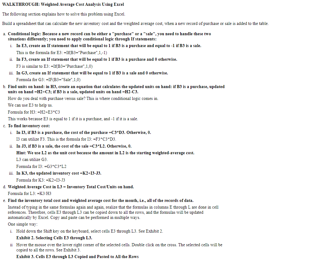
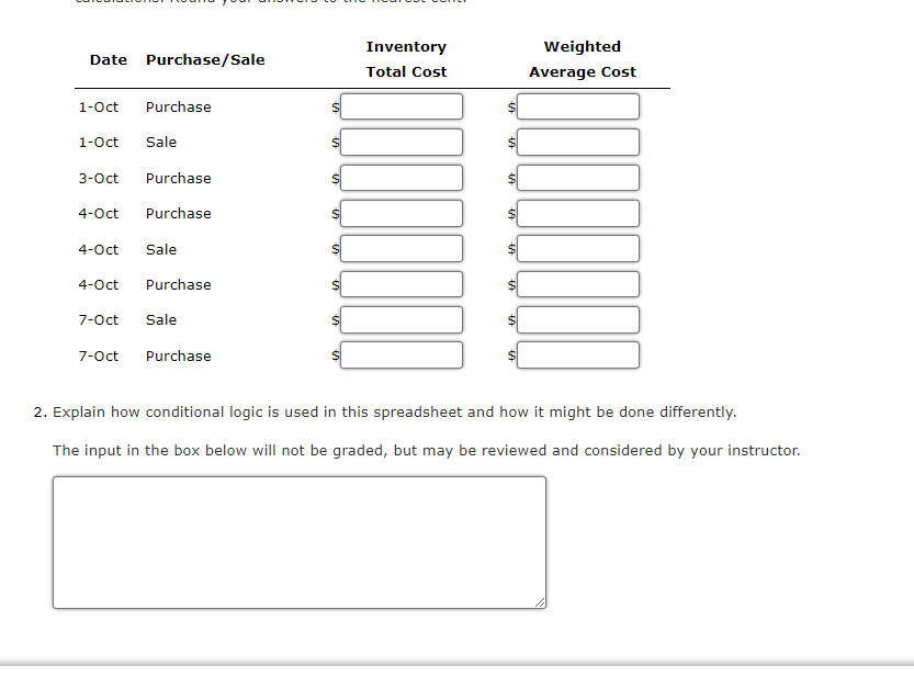
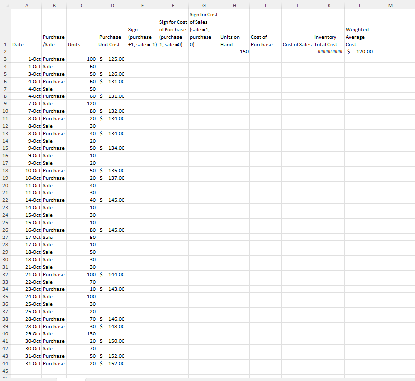
WALKTHROUGH: Weighted Average Cost Analysis Using Excel The following section explains how to solve this problem using Excel. Build a spreadsheet that can calculate the new inventory cost and the weighted average cost, when a new record of purchase or sale is added to the table. a. Conditional logic: Because a new record can be either a "purchase" or a "sale", you need to handle these two situations differently; you need to apply conditional logic through If statements: i. In E3, create an If statement that will be equal to 1 if B3 is a purchase and equal to -1 if B3 is a sale. This is the formula for E3: =If(B3="Purchase", 1,-1) ii. In F3, create an If statement that will be equal to 1 if B3 is a purchase and 0 otherwise. F3 is similar to E3: =If(B3="Purchase", 1,0) ii. In G3, create an If statement that will be equal to 1 if B3 is a sale and 0 otherwise. Formula for G3: =IF(B3="Sale",1,0) b. Find units on hand: in H3, create an equation that calculates the updated units on hand: if B3 is a purchase, updated units on hand =H2+C3; if B3 is a sale, updated units on hand =H2-C3. How do you deal with purchase versus sale? This is where conditional logic comes in. We can use E3 to help us. Formula for H3: =H2+E3*C3 This works because E3 is equal to 1 if it is a purchase, and -1 if it is a sale. c. To find inventory cost: i. In 13, if B3 is a purchase, the cost of the purchase =C3*D3. Otherwise, 0. 13 can utilize F3. This is the formula for 13: =F3*C3*D3 ii. In J3, if B3 is a sale, the cost of the sale =C3*L2. Otherwise, 0. Hint: We use L2 as the unit cost because the amount in L2 is the starting weighted-average cost. L3 can utilize G3. Formula for 13: =G3*C3*L2 iii. In K3, the updated inventory cost =K2+13-J3. Formula for K3: =K2+13-J3 d. Weighted Average Cost in L3 = Inventory Total Cost/Units on hand. Formula for L3: =K3/H3 e. Find the inventory total cost and weighted average cost for the month, i.e., all of the records of data. Instead of typing in the same formulas again and again, realize that the formulas in columns E through L are done in cell references. Therefore, cells E3 through L3 can be copied down to all the rows, and the formulas will be updated automatically by Excel. Copy and paste can be performed in multiple ways. One simple way: i. Hold down the Shift key on the keyboard, select cells E3 through L3. See Exhibit 2. Exhibit 2. Selecting Cells E3 through L3. ii Hover the mouse over the lower right corner of the selected cells. Double click on the cross. The selected cells will be copied to all the rows. See Exhibit 3. Exhibit 3. Cells E3 through L3 Copied and Pasted to All the RowsInventory Weighted Date Purchase/Sale Total Cost Average Cost 1-Oct purchase 1-Oct Sale 3-Oct Purchase 4-Oct Purchase 4-Oct Sale 4-Oct Purchase 7-Oct Sale 7-Oct Purchase 2. Explain how conditional logic is used in this spreadsheet and how it might be done differently. The input in the box below will not be graded, but may be reviewed and considered by your instructor.C G H K M B D E F Sign for Cost Sign for Cost of Sales Weighted Sign of Purchase (sale = 1, Cost of Inventory Average Purchase Purchase (purchase = (purchase = purchase= Units on Date /Sale Units Unit Cost +1, sale =-1) 1, sale =0) 0) Hand Purchase Cost of Sales Total Cost Cost 150 #WWWWWWWW# $ 120.00 1-Oct Purchase 100 $ 125.00 IM A W N 1 1-Oct Sale 60 3-Oct Purchase 50 5 126.00 4-Oct Purchase 50 5 131.00 4-Oct Sale 50 4-Oct Purchase 60 5 131.00 7-Oct Sale 120 10 7-Oct Purchase 80 5 132.00 11 8-Oct Purchase 20 5 134.00 12 8-Oct Sale 30 13 8-Oct Purchase 40 5 134.00 14 9-Oct Sale 20 15 9-Oct Purchase 50 5 134.00 16 9-Oct Sale 10 17 9-Oct Sale 20 18 10-Oct Purchase 50 5 135.00 19 10-Oct Purchase 20 5 137.00 20 11-Oct Sale 40 21 11-Oct Sale 30 22 14-Oct Purchase 40 5 145.00 23 14-Oct Sale 10 24 15-Oct Sale 30 25 15-Oct Sale 10 26 16-Oct Purchase 80 5 145.00 27 17-Oct Sale 50 28 17-Oct Sale 10 29 18-Oct Sale 50 30 18-Oct Sale 30 31 21-Oct Sale 30 32 21-Oct Purchase 100 5 144.00 33 22-Oct Sale 70 34 23-Oct Purchase 10 5 143.00 35 24-Oct Sale 100 36 25-Oct Sale 30 37 25-Oct Sale 20 28-Oct Purchase 70 5 146.00 39 28-Oct Purchase 30 5 148.00 40 29-Oct Sale 130 41 30-Oct Purchase 20 5 150.00 42 30-Oct Sale 70 43 31-Oct Purchase 5 152.00 44 31-Oct Purchase 20 5 152.00 45