Week 7

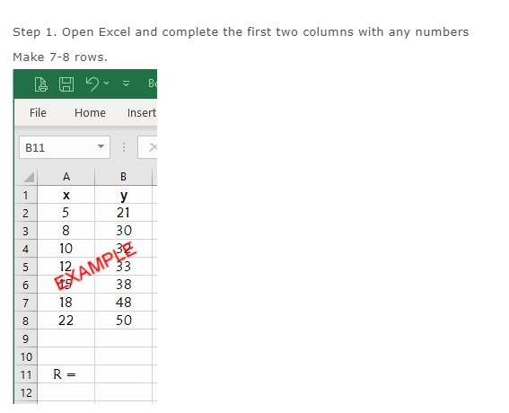
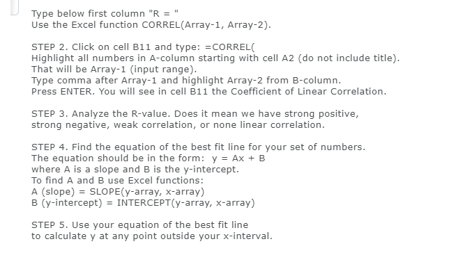
Step 1. Open Excel and complete the first two columns with any numbers Make 7-8 rows. B File Home Insert B11 A B X y 5 21 3 8 30 4 10 5 12 EXAMPLE 33 38 18 48 8 22 50 g 10 11 R = 12Type below rst column "R = "' Use the Excel function IZZIIEZIFtFtELUI'irray1,r Array2). STEP 2. Click on cell Ell and type: =CDRREL{ Highlight all numbers in Acolumn starting with cell A2 (do not include title}. That will be Array1 (input range}. Type comma after Array1 and highlight Array2 from Eicolumn. Press ENTER. You will see in cell I311 the Coefcient of Linear Correlation. STEP 3. hnalyze the Ryalue. Does it mean we have strong positive, strong negative, weak correlation, or none linear correlation. STEP 4. Find the equation of the best fit line for your set of numbers. The equation should be in the form: y = m: + E where P. is a slope and B is the yintercept. To nd A and El use Excel functions: A {slope} = SLOPE{yarray, antarray} B (yintercept} = INTERCEPT{yarray, xarray} STEP 5. Use your equation of the best fit line to calculate y at any point outside your xinteryal