Well-documented Jupyter Notebook script (.ipynb) should be included using python for the codes.

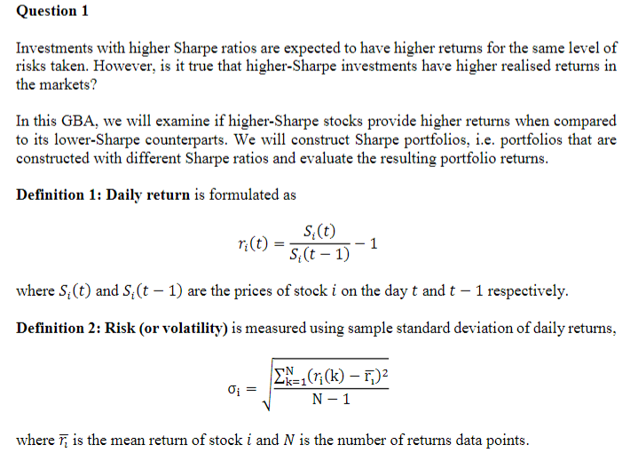
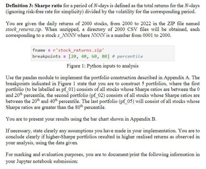
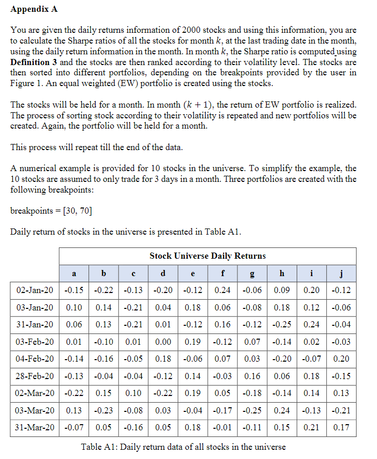
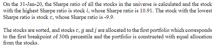
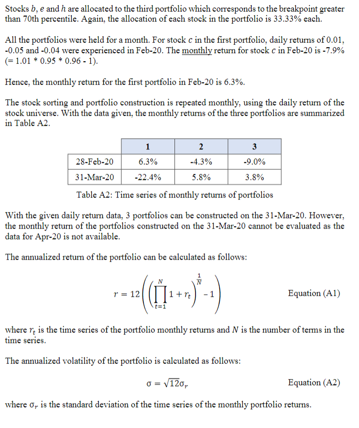
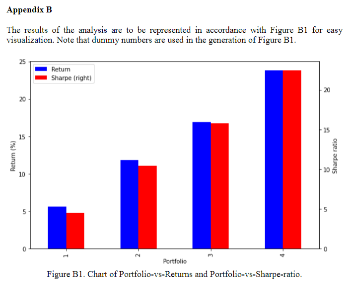
Investments with higher Sharpe ratios are expected to have higher returns for the same level of risks taken. However, is it true that higher-Sharpe investments have higher realised returns in the markets? In this GBA, we will examine if higher-Sharpe stocks provide higher returns when compared to its lower-Sharpe counterparts. We will construct Sharpe portfolios, i.e. portfolios that are constructed with different Sharpe ratios and evaluate the resulting portfolio returns. Definition 1: Daily return is formulated as ri(t)=Si(t1)Si(t)1 where Si(t) and Si(t1) are the prices of stock i on the day t and t1 respectively. Definition 2: Risk (or volatility) is measured using sample standard deviation of daily returns, i=N1k=1N(ri(k)r1)2 where rl is the mean return of stock i and N is the number of returns data points. Definition 3: Sharpe ratio for a period of N-days is defined as the total returns for the N-days (ignoring risk-free rate for simplicity) divided by the volatility for the corresponding period. You are given the daily returns of 2000 stocks, from 2000 to 2022 in the ZIP file named stock_returns.zip. When unzipped, a directory of 2000 CSV files will be obtained, each corresponding to a stock sNNNN where NNNN is a number from 0001 to 2000 . \[ \begin{array}{l} \text { fname }=r^{\prime} \text { stock_returns.zip' } \\ \text { breakpoints }=[20,40,60,80] \# \text { percentile } \end{array} \] Figure 1: Python inputs to analysis Use the pandas module to implement the portfolio construction described in Appendix A. The breakpoints indicated in Figure 1 state that you are to construct 5 portfolios, where the first portfolio (to be labelled as pf_01) consists of all stocks whose Sharpe ratios are between the 0 and 20th percentile, the second portfolio (pf_02) consists of all stocks whose Sharpe ratios are between the 20th and 40th percentile. The last portfolio (pf_05) will consist of all stocks whose Sharpe ratios are greater than the 80th percentile. You are to present your results using the bar chart shown in Appendix B. If necessary, state clearly any assumptions you have made in your implementation. You are to conclude clearly if higher-Sharpe portfolios resulted in higher realised returns as observed in your analysis, using the data given. For marking and evaluation purposes, you are to document/print the following information in your Jupyter notebook submission: You are given the daily returns information of 2000 stocks and using this information, you are to calculate the Sharpe ratios of all the stocks for month k, at the last trading date in the month, using the daily return information in the month. In month k, the Sharpe ratio is computed_using Definition 3 and the stocks are then ranked according to their volatility level. The stocks are then sorted into different portfolios, depending on the breakpoints provided by the user in Figure 1. An equal weighted (EW) portfolio is created using the stocks. The stocks will be held for a month. In month (k+1), the return of EW portfolio is realized. The process of sorting stock according to their volatility is repeated and new portfolios will be created. Again, the portfolio will be held for a month. This process will repeat till the end of the data. A numerical example is provided for 10 stocks in the universe. To simplify the example, the 10 stocks are assumed to only trade for 3 days in a month. Three portfolios are created with the following breakpoints: breakpoints =[30,70] Daily return of stocks in the universe is presented in Table A1. Table A1: Daily return data of all stocks in the universe On the 31-Jan-20, the Sharpe ratio of all the stocks in the universe is calculated and the stock with the highest Sharpe ratio is stock i, whose Sharpe ratio is 10.91. The stock with the lowest Sharpe ratio is stock c, whose Sharpe ratio is 9.9. The stocks are sorted, and stocks c,g and j are allocated to the first portfolio which corresponds to the first breakpoint of 30 th percentile and the portfolio is constructed with equal allocation from the stocks. Stocks b,e and h are allocated to the third portfolio which corresponds to the breakpoint greater than 70th percentile. Again, the allocation of each stock in the portfolio is 33.33% each. All the portfolios were held for a month. For stock c in the first portfolio, daily returns of 0.01, 0.05 and 0.04 were experienced in Feb-20. The monthly return for stock c in Feb-20 is 7.9% (=1.010.950.961) Hence, the monthly return for the first portfolio in Feb- 20 is 6.3%. The stock sorting and portfolio construction is repeated monthly, using the daily return of the stock universe. With the data given, the monthly returns of the three portfolios are summarized in Table A2. Table A2: Time series of monthly returns of portfolios With the given daily return data, 3 portfolios can be constructed on the 31-Mar-20. However, the monthly return of the portfolios constructed on the 31-Mar-20 cannot be evaluated as the data for Apr-20 is not available. The annualized return of the portfolio can be calculated as follows: r=12((t=1N1+rt)N11) Equation (A1) where rt is the time series of the portfolio monthly returns and N is the number of terms in the time series. The annualized volatility of the portfolio is calculated as follows: =12r Equation (A2) where r is the standard deviation of the time series of the monthly portfolio returns. The results of the analysis are to be represented in accordance with Figure B1 for easy visualization. Note that dummy numbers are used in the generation of Figure B1