What to press on excel step by step please.

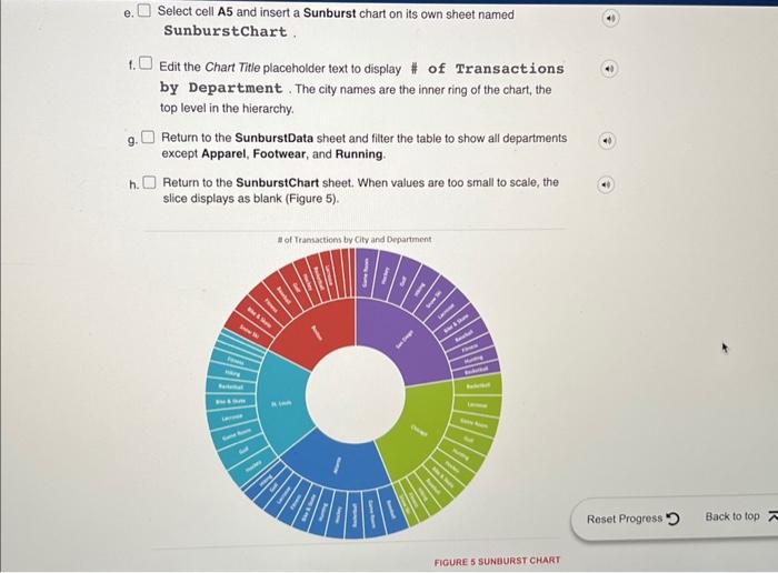
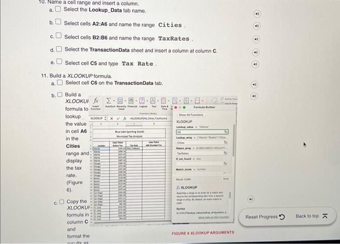
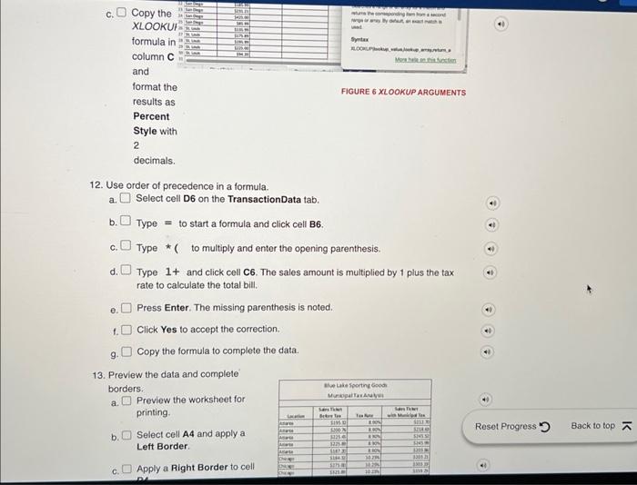
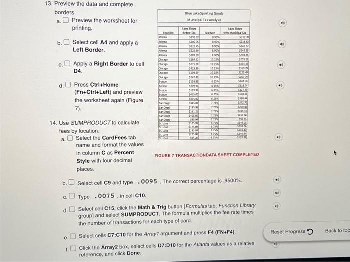
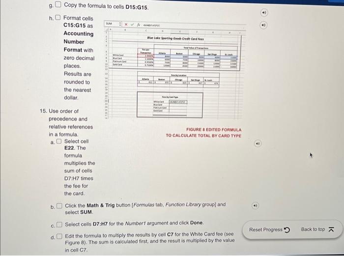
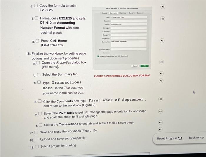
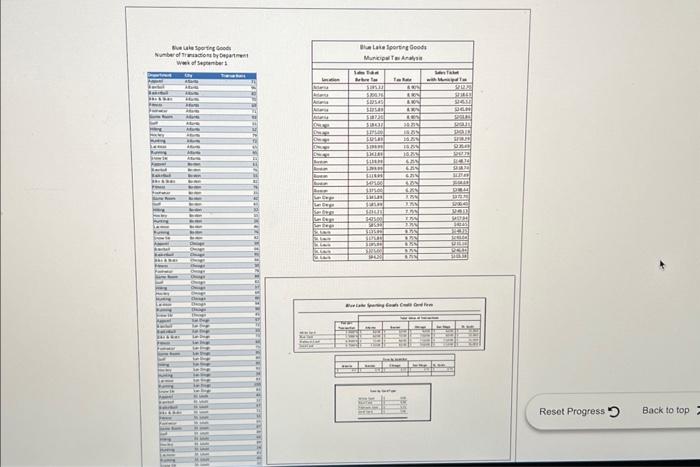
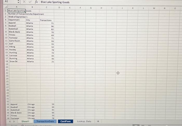
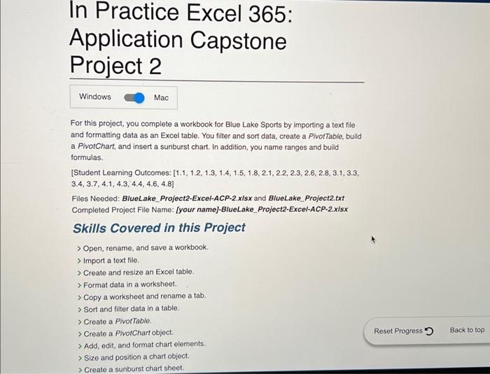
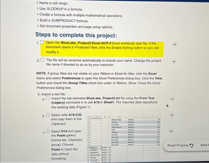
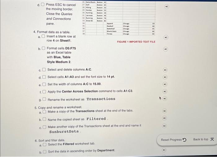
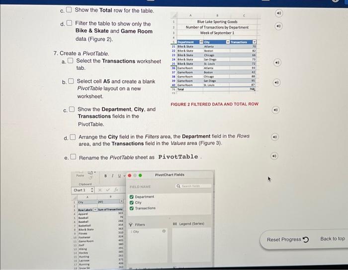
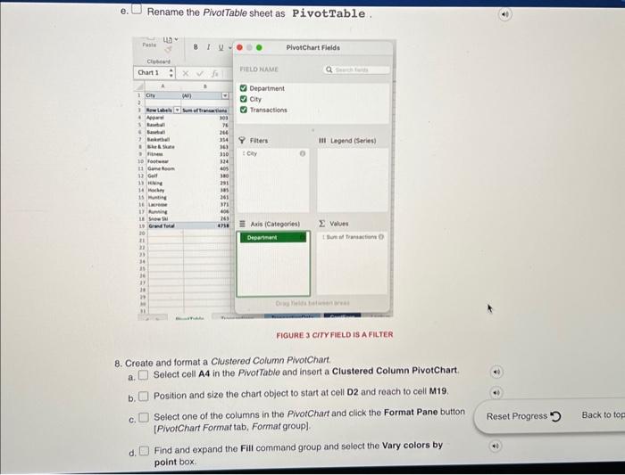
e. Copy the formula to cells E23:E25. f. Format cells E22:E25 and cells \\( \\mathrm{D} 7: \\mathrm{H} 10 \\) as Accounting Number Format with zero decimal places. g. Press \\( \\mathrm{Ctrl}+\\mathrm{Home} \\) (Fn+Ctri+Left). 6. Finalize the workbook by setting page options and document properties. a. Open the Properties dialog box [File menu]. b. Select the Summary tab. FIGURE 9 PROPERTIES DIALOG BOX FOR MAC c. Type Transactions Data in the Title box; type your name in the Author box. d. Click the Comments box, type First week of September. and return to the workbook (Figure 9). e. Select the PivotTable sheet tab. Change the page orientation to landscape and scale the sheet to fit a single page. e. Select cell A5 and insert a Sunburst chart on its own sheet named SunburstChart. 1. Edit the Chart Title placeholder text to display \\# of Transactions by Department. The city names are the inner ring of the chart, the top level in the hierarchy. g. Return to the SunburstData sheet and filter the table to show all departments except Apparel, Footwear, and Running. h. Return to the SunburstChart sheet. When values are too small to scale, the slice displays as blank (Figure 5). e. Close the Format Data Series task pane. f. Click the Total title box in the chart and edit the text to display \\# of Transactions by Department. g. Apply a Black, Text 1 outline with a weight of \\( 1 / 4 \\mathrm{pt} \\) to the chart object. h. Hide the display of Field Buttons in the PivotChart. Note: Mac users please skip this step and proceed to the next step. i. Select cell A21 (Figure 4). FIGURE 4 PINOTTABLE AND ITS CHART 9. Create and format a sunburst chart. a. Select the SunburstData tab name. b. Solect column B, cut it, and insert it at column \\( \\mathbf{A} \\) to rearrange the data so that the City column is column \\( A \\). The top level in a hierarchy chart should be leftmost in the data. c. Solect cells B1:B3 and move them to column A. d. Select cells A1:C3 and apply the Center Across Selection command. Ave uia loortin Coobs Woic of stpoumber: 13. Preview the data and complete borders. a. Preview the worksheet for printing. b. Select cell A4 and apply a Left Border. C. Apply a Right Border to cell D4. d. Press \\( \\mathrm{Ctrl}+\\mathrm{Home} \\) \\( (\\mathrm{Fn}+\\mathrm{Ctrl}+\\mathrm{Left}) \\) and preview the worksheet again (Figure 7). In Practice Excel 365: Application Capstone Project 2 For this project, you complete a workbook for Blue Lake Sports by importing a text file and formatting data as an Excel table. You filter and sort data, create a PivotTable, build a PivotChart, and insert a sunburst chart. In addition, you name ranges and build formulas. [Student Learning Outcomes: [1.1, 1.2, 1.3, 1.4, 1.5. 1.8, 2.1, 2.2, 2.3, 2.6, 2.8, 3.1, 3.3, \\( 3.4,3.7,4.1,4.3,4.4,4.6,4.8] \\) Files Needed: BlueLake_Project2-Excel-ACP-2.xlsx and BlueLake_Project2.txt Completed Project File Name: [your name]-BlueLake_Project2-Excel-ACP-2.xisx A1 \\( \\quad \\times \\quad f_{x} \\) Blue Lake Sporting Goods d. Press ESC to cancel the moving border. Close the Queries and Connections pane. 4. Format data as a table. a. Insert a blank row at row 4 on Sheet1. FIOURE 1 IMPORTED TEXT FILE b. Format cells D5:F75 as an Excel table with Blue, Table Style Medium 2. c. Select and delete columns A:C. d. Select cells \\( \\mathrm{A} 1: \\mathrm{A} 3 \\) and set the font size to \\( 14 \\mathrm{pt} \\). e. Set the width of columns \\( A: C \\) to 15.00 . 1. Apply the Center Across Selection command to cells A1:C3. 9. Rename the worksheet as Transactions 5. Copy and rename a worksheet. a. Make a copy of the Transactions sheet at the end of the tabs: b. Name the copled sheet as Filtered. c. Make another copy of the Transactions sheet at the end and name it SunburstData. 6. Sort and filter data. a. Select the Filtered worksheet tab. b. Sort the data in ascending order by Department. e. Rename the PivotTable sheet as PivotTable. FIGURE 3 CITYFIELD IS A FILTER 8. Create and format a Clustered Column PivotChart. a. Select cell A4 in the PivotTable and insert a Clustered Column PivotChart b. Position and size the chart object to start at cell D2 and reach to cell M19. c. Select one of the columns in the PivotChart and click the Format Pane button [PivotChart Format tab, Format group]. d. Find and expand the Fill command group and select the Vary colors by point box. 12. Use order of precedence in a formula. a. Select cell D6 on the TransactionData tab. b. \\( \\quad \\) Type \\( = \\) to start a formula and click cell \\( \\mathbf{B} 6 \\). c. Type * ( to multiply and enter the opening parenthesis. d. Type 1+ and click cell C6. The sales amount is multiplied by 1 plus the tax rate to calculate the total bill. e. Press Enter. The missing parenthesis is noted. f. Click Yes to accept the correction. g. Copy the formula to complete the data. 13. Preview the data and complete borders. a. Preview the worksheet for printing. b. Select cell A4 and apply a Left Border. c. Apply a Right Border to cell 10. Name a cell range and insert a column. a. Select the Lookup_Data tab name. b. Select cells A2:A6 and name the range Cities c. Select cells B2:B6 and name the range TaxRates . d. Select the TransactionData sheet and insert a column at column C. e. Select cell C5 and type Tax Rate . 11. Build a XLOOKUP formula. \\( > \\) Name a cell range. \\( > \\) Use XLOOKUP in a formula. \\( > \\) Create a formula with multiple mathematical operations. \\( > \\) Build a SUMPRODUCT formula. >Set document properties and page setup options. Steps to complete this project: 1. Open the BlueLake Project2-Excel-ACP-2 Excel workbook start file. If the document opens in Protected View, click the Enable Editing button so you can modify it. 2. The file will be renamed automatically to include your name. Change the project file name if directed to do so by your instructor. NOTE: If group titles are not visible on your Ribbon in Excel for Mac, click the Excel menu and select Preferences to open the Excel Preferences dialog box. Click the View button and check the Group Titles check box under In Ribbon, Show. Close the Excel Preferences dialog box. 3. Import a text file. a. Import the tab-delimited BlueLake_Project2.txt file using the From Text (Legacy) command in to cell A19 in Sheet1. The imported data repositions the existing data (Figure 1). c. Show the Total row for the table. d. Filter the table to show only the Bike \\& Skate and Game Room data (Figure 2). Copy the formula to cells D15:G15. Format cells C15:G15 as Accounting Number Format with zero decimal places. Results are rounded to the nearest dollar. order of ocedence and ative references a formula. Select cell E22. The formula multiplies the sum of cells D7:H7 times the fee for the card. Click the Math \\& Trig button [Formulas tab, Function Library group] and select SUM