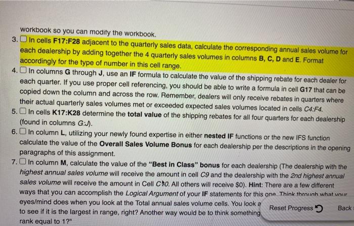
workbook so you can modify the workbook. 3. In cells F17:F28 adjacent to the quarterly sales data, calculate the corresponding annual sales volume for each dealership by adding together the 4 quarterly sales volumes in columns B, C, D and E. Format accordingly for the type of number in this cell range. 4. In columns G through J, use an IF formula to calculate the value of the shipping rebate for each dealer for each quarter. If you use proper cell referencing, you should be able to write a formula in cell G17 that can be copied down the column and across the row. Remember, dealers will only receive rebates in quarters where their actual quarterly sales volumes met or exceeded expected sales volumes located in cells C4:F4. 5. In cells K17:K28 determine the total value of the shipping rebates for all four quarters for each dealership (found in columns G:J). 6. In column L, utilizing your newly found expertise in either nested IF functions or the new IFS function calculate the value of the Overall Sales Volume Bonus for each dealership per the descriptions in the opening paragraphs of this assignment. 7. In column M, calculate the value of the "Best in Class" bonus for each dealership (The dealership with the highest annual sales volume will receive the amount in cell C9 and the dealership with the 2nd highest annual sales volume will receive the amount in Cell Cio. All others will receive $0). Hint: There are a few different ways that you can accomplish the Logical Argument of your IF statements for this one Think throunh what your eyes/mind does when you look at the Total annual sales volume cells. You look a Reset Progress Back to see if it is the largest in range, right? Another way would be to think something rank equal to 1?" workbook so you can modify the workbook. 3. In cells F17:F28 adjacent to the quarterly sales data, calculate the corresponding annual sales volume for each dealership by adding together the 4 quarterly sales volumes in columns B, C, D and E. Format accordingly for the type of number in this cell range. 4. In columns G through J, use an IF formula to calculate the value of the shipping rebate for each dealer for each quarter. If you use proper cell referencing, you should be able to write a formula in cell G17 that can be copied down the column and across the row. Remember, dealers will only receive rebates in quarters where their actual quarterly sales volumes met or exceeded expected sales volumes located in cells C4:F4. 5. In cells K17:K28 determine the total value of the shipping rebates for all four quarters for each dealership (found in columns G:J). 6. In column L, utilizing your newly found expertise in either nested IF functions or the new IFS function calculate the value of the Overall Sales Volume Bonus for each dealership per the descriptions in the opening paragraphs of this assignment. 7. In column M, calculate the value of the "Best in Class" bonus for each dealership (The dealership with the highest annual sales volume will receive the amount in cell C9 and the dealership with the 2nd highest annual sales volume will receive the amount in Cell Cio. All others will receive $0). Hint: There are a few different ways that you can accomplish the Logical Argument of your IF statements for this one Think throunh what your eyes/mind does when you look at the Total annual sales volume cells. You look a Reset Progress Back to see if it is the largest in range, right? Another way would be to think something rank equal to 1