Write the equation with the dependent variable of the log return and the independent variables of the cutoff, agreed terms AR and MA;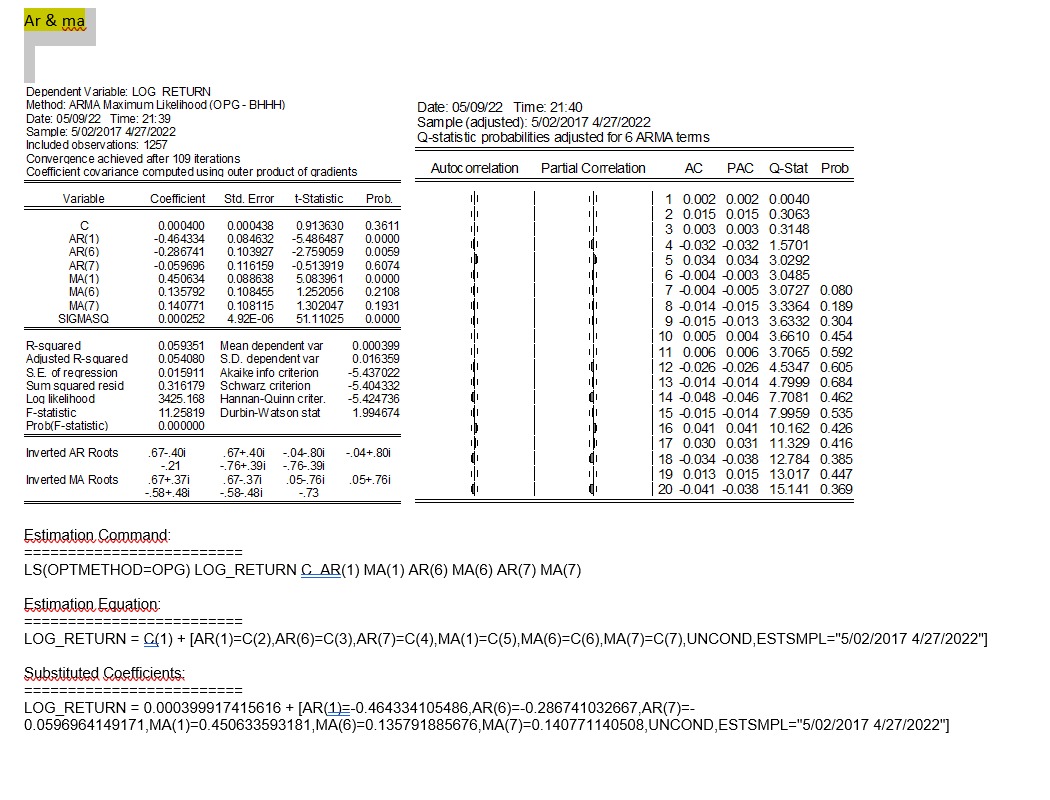

Ar & ma - Date: 05/09/22 Time: 21:40 Sample (adjusted): 5/02/2017 4/27/2022 Q-statistic probabilities adjusted for 6 ARMA tems Autocorrelation Partial Correlation AC PAC Q-Stat Prob Prob. li oli Dependent Variable: LOG RETURN Method: ARMA Maximum Likelihood (OPG-BHHH) Date: 05/09/22 Time: 21:39 Sample: 5/02/2017 4/27/2022 Included observations: 1257 Convergence achieved after 109 iterations Coefficient covariance computed using outer product of gradients Variable Coefficient Std. Error t-Statistic 0.000400 0.000438 0.913630 AR(1) -0.464334 0.084632 -5.486487 AR(6) -0.286741 0.103927 -2.759059 AR(7) -0.059696 0.116159 -0.513919 MA(1) 0.450634 0.088638 5.083961 MA(6) 0.135792 0.108455 1.252056 MA(7) 0.140771 0.108115 1.302047 SIGMASQ 0.000252 4.92E-06 51.11025 10 0.3611 0.0000 0.0059 0.6074 0.0000 0.2108 0.1931 0.0000 111 R-squared Adjusted R-squared S.E. of regression Sum squared resid Log likelihood F-statistic Prob(F-statistic) 0.059351 Mean dependent var 0.054080 S.D. dependent var 0.015911 Akaike info criterion 0.316179 Schwarz criterion 3425.168 Hannan-Quinn criter 11.25819 Durbin-Watson stat 0.000000 0.000399 0.016359 -5.437022 -5.404332 -5.424736 1.994674 1 0.002 0.002 0.0040 2 0.015 0.015 0.3063 3 0.003 0.003 0.3148 4 0.032 0.032 1.5701 5 0.034 0.034 3.0292 6 0.004 -0.003 3.0485 70.004 0.005 3.0727 0.080 8 -0.014 0.015 3.3364 0.189 9 -0.015 -0.013 3.6332 0.304 10 0.005 0.004 3.6610 0.454 11 0.006 0.006 3.7065 0.592 12 0.026 0.026 4.5347 0.605 13 0.014 0.014 4.7999 0.684 14 0.048 0.046 7.7081 0.462 18 15 0.015 0.014 7.9959 0.535 100 101 16 0.041 0.041 10.162 0.426 17 0.030 0.031 11.329 0.416 18 0.034 0.038 12.784 0.385 19 0.013 0.015 13.017 0.447 20 0.041 0.038 15.141 0.369 Inverted AR Roots -.04+ 801 .67-401 -21 .67+ 371 - 58+ 481 .67+ 401 -.76+. 39 67-371 -58-.481 -04-.80i -76-39 .05-.761 -.73 Inverted MA Roots .05+.761 Estimation Command: LS(OPTMETHOD=OPG) LOG_RETURN C AR(1) MA(1) AR(6) MA(6) AR(7) MA(7) Estimation Equation: ========= LOG_RETURN = C(1) + [AR(1)=C(2),AR(6)=C(3), AR(7)=C(4), MA (1)=C(5),MA(6)=C(6),MA(7)=C(7), UNCOND, ESTSMPL="5/02/2017 4/27/2022"] = --========= Substituted Coefficients: ========= LOG_RETURN = 0.000399917415616 + [AR(1=-0.464334105486, AR(6)=-0.286741032667,AR(7)=- 0.0596964149171,MA(1)=0.450633593181,MA(6)=0.135791885676,MA(7)=0.140771140508, UNCOND,ESTSMPL="5/02/2017 4/27/2022"] Ar & ma - Date: 05/09/22 Time: 21:40 Sample (adjusted): 5/02/2017 4/27/2022 Q-statistic probabilities adjusted for 6 ARMA tems Autocorrelation Partial Correlation AC PAC Q-Stat Prob Prob. li oli Dependent Variable: LOG RETURN Method: ARMA Maximum Likelihood (OPG-BHHH) Date: 05/09/22 Time: 21:39 Sample: 5/02/2017 4/27/2022 Included observations: 1257 Convergence achieved after 109 iterations Coefficient covariance computed using outer product of gradients Variable Coefficient Std. Error t-Statistic 0.000400 0.000438 0.913630 AR(1) -0.464334 0.084632 -5.486487 AR(6) -0.286741 0.103927 -2.759059 AR(7) -0.059696 0.116159 -0.513919 MA(1) 0.450634 0.088638 5.083961 MA(6) 0.135792 0.108455 1.252056 MA(7) 0.140771 0.108115 1.302047 SIGMASQ 0.000252 4.92E-06 51.11025 10 0.3611 0.0000 0.0059 0.6074 0.0000 0.2108 0.1931 0.0000 111 R-squared Adjusted R-squared S.E. of regression Sum squared resid Log likelihood F-statistic Prob(F-statistic) 0.059351 Mean dependent var 0.054080 S.D. dependent var 0.015911 Akaike info criterion 0.316179 Schwarz criterion 3425.168 Hannan-Quinn criter 11.25819 Durbin-Watson stat 0.000000 0.000399 0.016359 -5.437022 -5.404332 -5.424736 1.994674 1 0.002 0.002 0.0040 2 0.015 0.015 0.3063 3 0.003 0.003 0.3148 4 0.032 0.032 1.5701 5 0.034 0.034 3.0292 6 0.004 -0.003 3.0485 70.004 0.005 3.0727 0.080 8 -0.014 0.015 3.3364 0.189 9 -0.015 -0.013 3.6332 0.304 10 0.005 0.004 3.6610 0.454 11 0.006 0.006 3.7065 0.592 12 0.026 0.026 4.5347 0.605 13 0.014 0.014 4.7999 0.684 14 0.048 0.046 7.7081 0.462 18 15 0.015 0.014 7.9959 0.535 100 101 16 0.041 0.041 10.162 0.426 17 0.030 0.031 11.329 0.416 18 0.034 0.038 12.784 0.385 19 0.013 0.015 13.017 0.447 20 0.041 0.038 15.141 0.369 Inverted AR Roots -.04+ 801 .67-401 -21 .67+ 371 - 58+ 481 .67+ 401 -.76+. 39 67-371 -58-.481 -04-.80i -76-39 .05-.761 -.73 Inverted MA Roots .05+.761 Estimation Command: LS(OPTMETHOD=OPG) LOG_RETURN C AR(1) MA(1) AR(6) MA(6) AR(7) MA(7) Estimation Equation: ========= LOG_RETURN = C(1) + [AR(1)=C(2),AR(6)=C(3), AR(7)=C(4), MA (1)=C(5),MA(6)=C(6),MA(7)=C(7), UNCOND, ESTSMPL="5/02/2017 4/27/2022"] = --========= Substituted Coefficients: ========= LOG_RETURN = 0.000399917415616 + [AR(1=-0.464334105486, AR(6)=-0.286741032667,AR(7)=- 0.0596964149171,MA(1)=0.450633593181,MA(6)=0.135791885676,MA(7)=0.140771140508, UNCOND,ESTSMPL="5/02/2017 4/27/2022"]