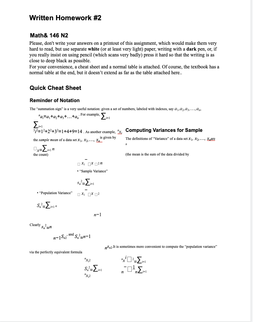
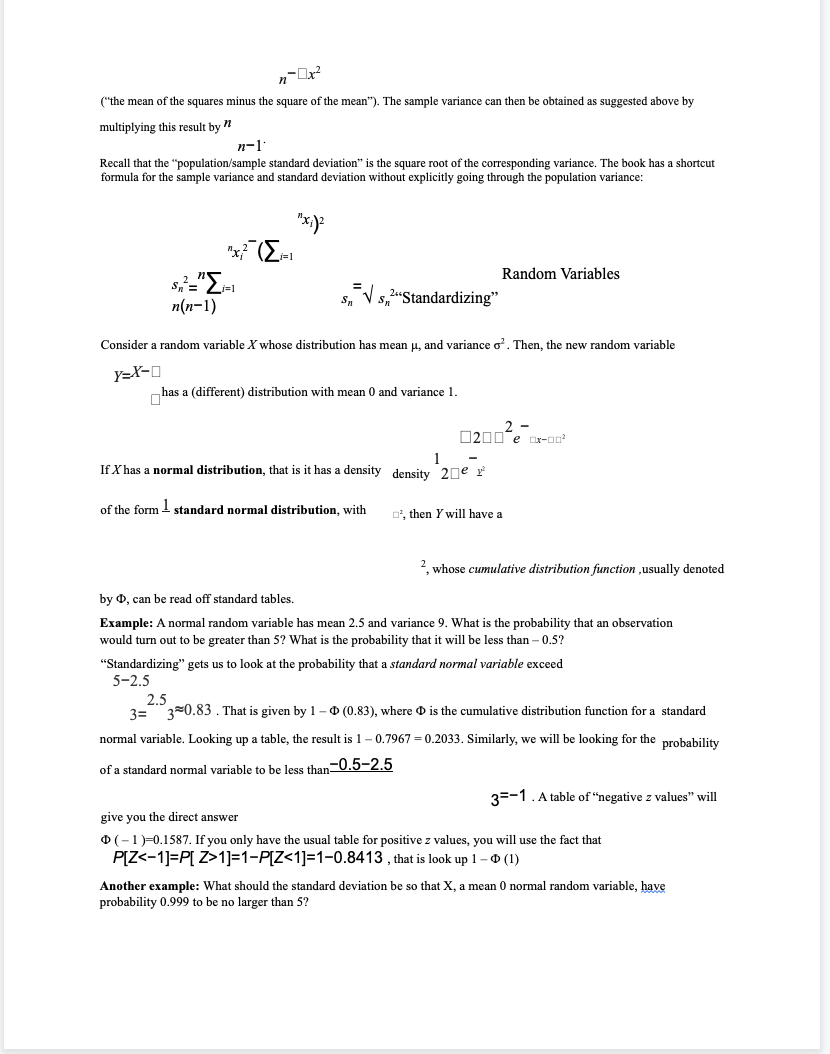
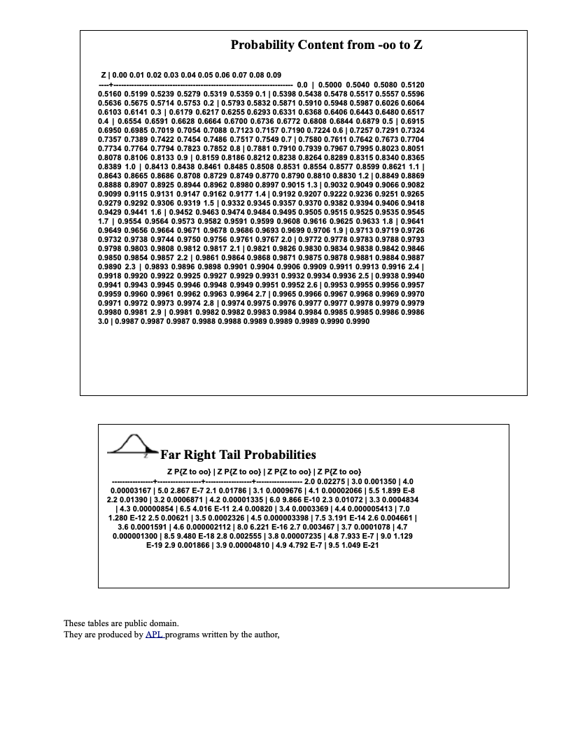
Written Homework #2 Math& 146 N2 Please, don't write your answers on a printout of this assignment, which would make them very hard to read, but use separate white (or at least very light) paper, writing with a dark pen, or, if you really insist on using pencil (which scans very badly) press it hard so that the writing is as close to deep black as possible. For your convenience, a cheat sheet and a normal table is attached. Of course, the textbook has a normal table at the end, but it doesn't extend as far as the table attached here.. Quick Cheat Sheet Reminder of Notation The "summation sign" is a very useful notation: given a set of numbers, labeled with indexes, say a, a ... "a=a+a+a+...+an i=1 For example, -1 32=12+22+32=1+4+9=14. As another example, "x Computing Variances for Sample the sample mean of a data set X1, X2, is given by The definitions of "Variance" of a data set X1, X2,..., Xare the count) 2 X X . "Sample Variance" i=1 "Population Variance" Xix2 n-1 (the mean is the sum of the data divided by Clearly 2 Sn=n n-1S2 and S=n-1 via the perfectly equivalent formula ns2.It is sometimes more convenient to compute the "population variance" "xp i=1 1*3"-" x2 ("the mean of the squares minus the square of the mean"). The sample variance can then be obtained as suggested above by multiplying this result by " n-1 Recall that the "population/sample standard deviation" is the square root of the corresponding variance. The book has a shortcut formula for the sample variance and standard deviation without explicitly going through the population variance: i=1 " n(n-1) Random Variables Sn ,"Standardizing" Consider a random variable X whose distribution has mean , and variance o. Then, the new random variable y=X- has a (different) distribution with mean 0 and variance 1. 2- 200e ox-00 1 If X has a normal distribution, that is it has a density density 2 of the form standard normal distribution, with , then I will have a 2, whose cumulative distribution function, usually denoted by D, can be read off standard tables. Example: A normal random variable has mean 2.5 and variance 9. What is the probability that an observation would turn out to be greater than 5? What is the probability that it will be less than -0.5? "Standardizing" gets us to look at the probability that a standard normal variable exceed 5-2.5 2.5 3= 30.83. That is given by 1 - D (0.83), where D is the cumulative distribution function for a standard normal variable. Looking up a table, the result is 1-0.7967-0.2033. Similarly, we will be looking for the probability of a standard normal variable to be less than- n-0.5-2.5 give you the direct answer 3=-1. A table of negative z values" will (-1)=0.1587. If you only have the usual table for positive z values, you will use the fact that P[Z 1]=1-P[Z