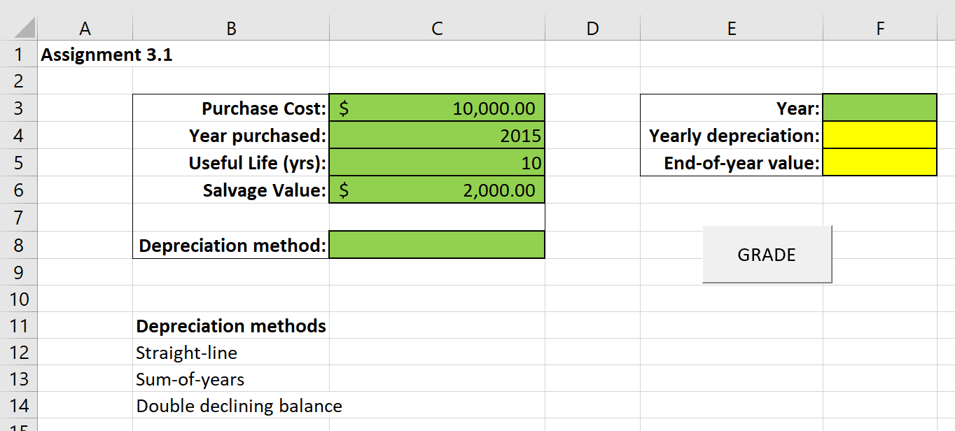you will create a worksheet that allows the user to input the Purchase Cost (in $), Year purchased , Useful Life (in years), and Salvage Value (in $), all in separate cells of the worksheet. Then, the user will select the Depreciation method from a drop-down list (data validation) in cell C8 . The depreciation methods available in the list are the 3 methods in cells B12: B14 ( Depreciation methods ), and it is important that the methods that show up in cell C8 are spelled exactly as they are in cells B12: B14 (the grader file will not work if you have misspelled these methods!). The user can then select a Year from the right side of the worksheet (cell F3 ) and the Yearly depreciation and End-of-year value for that asset for the corresponding Year will be displayed in cells F4 and F5 , respectively. IMPORTANTLY, the options that show up for Year in cell F3 will start with 1 year after the Year purchased in cell C4 and will go up to the number of years of Useful Life in cell C5 . For example, in the example shown below, the options available in the drop-down list in cellF3 would be 2016, 2017, 2018, ..., 2024, 2025 (only those 10 years, no more, no less). You can assume that the Useful Life is limited to 20 years (ie, the grader file will not put in anything greater than 20 in cell C5 ). It is also important that you don't move the location of any of the boxed in cells on the starter file!

HINTS:

• I had to create several (8) "helper" columns over to the right side of the worksheet. Afterwards, it is easy to hide these columns, if you wish.

• I would recommend using the OFFSET function in combination with the Useful Life value in your data validation List (you will want to use a formula) for cell F3 . You will also somehow (several ways to do this) account for the Year purchased (cell C4). If you have Office 365, you might look into using the SEQUENCE function.

• My formulas in cells F4 and F5 involved the following functions: MATCH , OFFSET , INDEX . These formulas referenced my "helper" columns.