

Question: It is not hard, with modern computing power, to solve the time-dependent Schrdinger equation in one dimension using an iterative approach. We define the wave
It is not hard, with modern computing power, to solve the time-dependent Schrödinger equation in one dimension using an iterative approach. We define the wave function ψ(x, t) on a set of discrete points x separated by distance dx, and update ψ(x, t) for a series of time steps dt according to the rule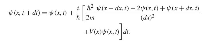
Use a program like Mathematica or MATLAB to define ψ(x, t) on a array of several hundred x points. To simulate an infinite system, use the periodic boundary condition ψ(L, t) = ψ(0, t), where L = Ndx is the length of the x region. Start the simulation with ψ(x, 0) = e−x2/l2, where l ≪ L, and V = 0, and pick a time interval dt small enough to see the evolution of the wave from a Gaussian peak to a constant spread through all space, as shown in Figure 9.21(a). For convenience, set h̄ = m = 1.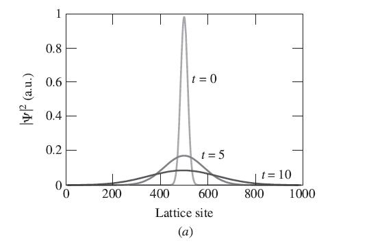
Next, let V(x) be a random field, in which the value at each x is chosen randomly, independent of the value at any other x. Evolve the wave function in this potential. You should see that, consistent with the discussion of Anderson localization in this section, the wave function does not spread out evenly, but remains bunched near x = 0 at all later times, as shown in Figure 9.21(b).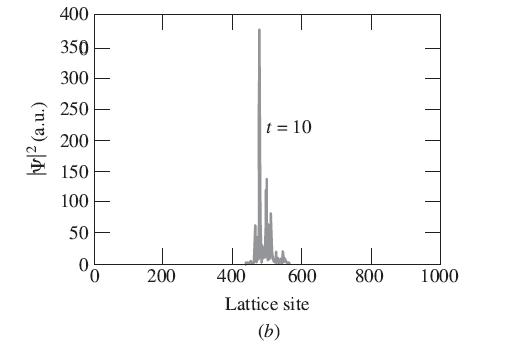
(x, t + dt) = (x, t) + i [ (x-dx, t) 2(x, t) + y(x + dx, t) h 2m (dx) +V(x)/(x, t) dt.
Step by Step Solution
3.44 Rating (151 Votes )
There are 3 Steps involved in it
In order to simplify the problem we separate the imaginary and real parts of the equation as Vr t ox t ixx t so we get a coupled set of two equations ... View full answer

Get step-by-step solutions from verified subject matter experts