For our running Example 2.

2 we can use (2.53) to derive a large-sample approximation of the pointwise variance of the learner \(g_{\mathscr{T}}(\boldsymbol{x})=\boldsymbol{x}^{\top} \widehat{\boldsymbol{\beta}}_{n}\). In particular, show that for large \(n\)

\[ \mathbb{V} \operatorname{ar} g_{\mathscr{T}}(\boldsymbol{x}) \simeq \frac{\ell^{*} \boldsymbol{x}^{\top} \mathbf{H}_{p}^{-1} \boldsymbol{x}}{n}+\frac{\boldsymbol{x}^{\top} \mathbf{H}_{p}^{-1} \mathbf{M}_{p} \mathbf{H}_{p}^{-1} \boldsymbol{x}}{n}, \quad n \rightarrow \infty \]
Figur 2.

18 shows this (large-sample) variance of the learner for different values of the predictor \(u\) and model index \(p\). Observe that the variance ultimately increases in \(p\) and that it is smaller at \(u=1 / 2\) than closer to the endpoints \(u=0\) or \(u=1\). Since the bias is also larger near the endpoints, we deduce that the pointwise mean squared error (2.21) is larger near the endpoints of the interval \([0,1]\) than near its middle. In other words, the error is much smaller in the center of the data cloud than near its periphery.

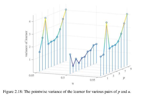
variance of learner 0.05 0.5 0.95 Figure 2.18: The pointwise variance of the learner for various pairs of p and u.