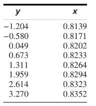
The article "Two Different Approaches for RDC Modelling When Simulating a Solvent Deasphalting Plant" (J. Aparicio, M. Heronimo, et al., Computers and Chemical Engineering, 2002:1369-1377) reports flow rate (in \(\mathrm{dm}^{3} / \mathrm{h}\) ) and specific gravity measurements for a sample of paraffinic hydrocarbons. The natural logs of the flow rates \((y)\) and the specific gravity measurements \((x)\) are presented in the following table.

a. Fit the linear model \(y=\beta_{0}+\beta_{1} x+\varepsilon\). For each coefficient, test the hypothesis that the coefficient is equal to 0 .

b. Fit the quadratic model \(y=\beta_{0}+\beta_{1} x+\beta_{2} x^{2}+\varepsilon\). For each coefficient, test the hypothesis that the coefficient is equal to 0 .

c. Fit the cubic model \(y=\beta_{0}+\beta_{1} x+\beta_{2} x^{2}+\beta_{3} x^{3}+\varepsilon\). For each coefficient, test the hypothesis that the coefficient is equal to 0 .

d. Which of the models in parts (a) through (c) is the most appropriate? Explain.

e. Using the most appropriate model, estimate the flow rate when the specific gravity is 0.83 .

y - 1.204 -0.580 0.049 0.673 1.311 1.959 2.614 3.270 X 0.8139 0.8171 0.8202 0.8233 0.8264 0.8294 0.8323 0.8352