New Semester Started Get 50% OFF Study Help! --h --m --s Claim Now

Question Answers

Textbooks

Find textbooks, questions and answers

Oops, something went wrong!

Change your search query and then try again

Result Not Found

Books FREE
Study Help
Tutors
AI Study Planner NEW
Sell Books

Search
Sign In
Register

study help
mathematics
statistics

Statistical Inference 2nd edition George Casella, Roger L. Berger - Solutions

In Theorem 2.1.10 the probability integral transform was proved, relating the uniform cdf to any continuous cdf. In this exercise we investigate the relationship between discrete random variables and uniform random variables. Let X be a discrete random variable with cdf Fx(x) and define the random
Let X have the standard normal pdf, fx(x) = (l/√2π)e-x2/2. (a) Find EX2 directly, and then by using the pdf of Y = X2 from Example 2.1.7 and calculating E Y. (b) Find the pdf of Y = |X|, and find its mean and variance.
A random right triangle can be constructed in the following manner. Let A be a random angle whose distribution is uniform on (0,Ï€/2). For each X, construct a triangle as pictured below. Here, Y = height of the random triangle. For a fixed constant d, find the distribution of Y and EY.
Consider a sequence of independent coin flips, each of which has probability p of being heads. Define a random variable X as the length of the run (of either heads or tails) started by the first trial. (For example, X = 3 if either TTTH or HHHT is observed.) Find the distribution of X, and find EX.
(a) Let X be a continuous, nonnegative random variable [f(x) = 0 for xwhere Fx(x) is the cdf of X. (b) Let X be a discrete random variable whose range is the nonnegative integers. Show that where Fx(k) - P(X ‰¤ k). Compare this with part (a).
Betteley (1977) provides an interesting addition law for expectations. Let X and Y be any two random variables and define X ∧ Y = min(X, Y) and X V Y = max(X, Y). Analogous to the probability law P(A ∪ B) = P(A) + P(B) - P(A ∩ B), show that E(X V Y) = EX + E Y - E(X A Y).
Use the result of Exercise 2.14 to find the mean duration of certain telephone calls, where we assume that the duration, T, of a particular call can be described probabilistically by P(T > t) = ae-λt + (1 - a)e-μt, where a, A, and p are constants, 0 < a < 1, λ > 0, μ > 0.
A median of a distribution is a value m such that P(X ‰¤ m) ‰¥ 1/2 and P(X ‰¥ m) ‰¥ 1/2.(If X is continuous, m satisfiesFind the median of the following distributions. (a) f(x) = 3x2, 0 (b)
Show that if X is a continuous random variable, thenwhere m is the median of X (see Exercise 2.17),
Prove thatby differentiating the integral. Verify, using calculus, that a = EX is indeed a minimum. List the assumptions about Fx and fx that are needed.
In each of the following find the pdf of Y.(a) y = X2 and fx(x) = 1, 0 (b) y = - log X and X has pdf (c) Y = ex and X has pdf
A couple decides to continue to have children until a daughter is born. What is the expected number of children of this couple?
Prove the "two-way" rule for expectations, equation (2.2.5), which says E g(X) = E Y, where Y = g(X). Assume that g(x) is a monotone function.
Let X have the pdf(a) Verify that f(x) is a pdf. (b) Find EX and Var X.
Let X have the pdf(a) Find the pdf of Y = X2 (b) Find EY and Var Y.
Compute EX and Var X for each of the following probability distributions. (a) fx(x) =αxa-1,0 < x < l, a>0 (b) fx(x) = 1/n, 2,..., n, n > 0 an integer (c) fx(x) = 3/2 (x - l)2, 0 < x < 2
Suppose the pdf fx(x) of a random variable X is an even function. (fx(x) is an even function if fx(x) = fx(-x) for every x.) Show that (a) X and -X are identically distributed. (b) Mx(t) is symmetric about 0.
Let f(x) be a pdf and let a be a number such that, for all ∈ > 0, f(a + ∈) = f(a - ∈). Such a pdf is said to be symmetric about the point a. (a) Give three examples of symmetric pdfs. (b) Show that if X ~ f(x), symmetric, then the median of X (see Exercise 2.17) is the number a. (c) Show that
Let f(x) be a pdf, and let a be a number such that if a ≥ x ≥ y, then f(a) ≥ f(x) ≥ f(y), and if a ≤ x ≤ y, then f(a) ≥ f(x) ≥ f(y). Such a pdf is called unimodal with a mode equal to a. (a) Give an example of a unimodal pdf for which the mode is unique. (b) Give an example of a
Let Î¼n denote the nth central moment of a random variable X. Two quantities of interest, in addition to the mean and variance, areThe value Î±3 is called the skewness and ou is called the kurtosis. The skewness measures the lack of symmetry in the pdf (see Exercise 2.26).
To calculate moments of discrete distributions, it is often easier to work with the factorial moments (see Miscellanea 2.6.2).(a) Calculate the factorial moment E[X (X - 1)] for the binomial and Poisson distributions.(b) Use the results of part (a) to calculate the variances of the binomial and
Suppose X has the geometric pmf fx(x) = 1/3 (2/3)x, x = 0,1,2,- Determine the probability distribution of Y = X/(X + 1). Here both X and Y are discrete random variables. To specify the probability distribution of Y, specify its pmf.
Find the moment generating function corresponding to(a) f(x) = 1/c, 0 (b) f(x) = 2x/c2, 0 (c) f(x) = 1/2Î² e-|x - Î±| Î², - ˆž 0.(d)
Does a distribution exist for which Mx(t) = t/( 1 - t), |t| < 1? If yes, find it. If no, prove it.
Let Mx(t) be the moment generating function of X, and define S(t) = log(Mx(t)). Show that
In each of the following cases verify the expression given for the moment generating function, and in each case use the mgf to calculate E X and Var X.
Fill in the gaps in Example 2.3.10.(a) Show that if X1~ f1(x), thenEXrl = er2/2, r = 0,1,....So f1 (x) has all of its moments, and all of the moments are finite.(b) Now show thatfor all positive integers r, so EXr1 = EXr2 for all r. (Romano and Siegel 1986 discuss an extreme version of this
The lognormal distribution, on which Example 2.3.10 is based, has an interesting property. If we have the pdfthen Exercise 2.35 shows that all moments exist and sire finite. However, this distribution does not have a moment generating function, that is, does not exist. Prove this.
Referring to the situation described in Miscellanea 2.6.3: (a) Plot the pdfs f1 and f2 to illustrate their difference. (b) Plot the cumulant generating functions K1 and K2 to illustrate their similarity. (c) Calculate the moment generating functions of the pdfs f1 and f2. Are they similar or
In each of the following cases calculate the indicated derivatives, justifying all operations.(a)(b) (c) (d)
Let A be a fixed positive constant, and define the function f(x) by f(x) = 1/2 λe- λx if x > 0 and f(x) = 1/2 λeλx if x < 0. (a) Verify that f(x) is a pdf. (b) If A" is a random variable with pdf given by /(x), find P(X < t) for all t. Evaluate all integrals. (c) Find P(|X| < t) for all t.
Use Theorem 2.1.8 to find the pdf of Y in Example 2.1.2. Show that the same answer is obtained by differentiating the cdf given in (2.1.6).
In each of the following find the pdf of Y and show that the pdf integrates to 1. (a) fx(x) = 1/2e-|x|, -∞ < x < ∞; Y = |X|3 (b) fx(x) = 3/8(x + l)2, -1 < x < 1; Y = 1 - x2 (c) fx(x) = 3/8(x+ l)2, -1 < x < 1; Y = 1 - X2 if X ≤ 0 and Y = 1 - X if X > 0
Let X have pdf fx(x) = 2/9(x + 1), - 1 < x < 2. (a) Find the pdf of Y = X2. Theorem 2.1.8 is not directly applicable in this problem. (b) Show that Theorem 2.1.8 remains valid if the sets A0, A1,..., Ak, contain X, and apply the extension to solve part (a) using A0 = θ, A1 = (-2,0), and A2 = (0,2).
In each of the following show that the given function is a cdf and find F-1x(y)(a)(b) (c) In part (c), Fx(x) is discontinuous but (2.1.13) is still the appropriate definition of F-1x(y).
If the random variable X has pdffind a monotone function it(x) such that the random variable Y = u(X) has a uniform(0,1) distribution.
Find experience for EX and Vax X if X is a random variables with the general discrete uniform(N0, N1) distribution that puts equal probability in each of the values N0, N0 + 1, . . . . . . . . . ., N1. Here N0 < and both are integers
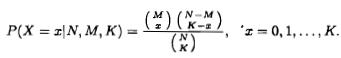
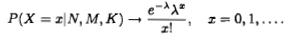
The hypergeometric distribution can be approximated by either the binomial or the Poisson distribution. (Of course, it can be approximated by other distributions, but in this exercise we will concentrate on only these two.) Let X have the hypergeometric distribution(a) Show that as N → ∞,
Suppose X has a binomial(n, p) distribution and let Y have a negative binomial(r, p) distribution. Show that Fx(r - 1) = 1 - Fy(n - r).
A truncated discrete distribution is one in which a particular class cannot be observed and is eliminated from the sample space. In particular, if X has range 0, 1, 2,... and the 0 class cannot be observed (as is usually the case), the O-truncated random variable XT has pmfFind the pmf, mean, and
Starting from the O-truncated negative binomial (refer to Exercise 3.13), if we let r †’ 0, we get an interesting distribution, the logarithmic series distribution. A random variable X has a logarithmic series distribution with parameter p if(a) Verify that this defines a legitimate
In Section 3.2 it was claimed that the Poisson(A) distribution is the limit of the negative binomial(r, p) distribution as r → ∞, p → 1, and r(l - p) → λ. Show that under these conditions the mgf of the negative binomial converges to that of the Poisson.
Verify these two identities regarding the gamma function that were given in the text: (a) Г(a +1) = aГ(a) (b) Г(1/2) = √π
Establish a formula similar to (3.3.18) for the gamma distribution. If X ~ gamma(Î±, Î²), then for any positive constant v,
There is an interesting relationship between negative binomial and gamma random variables, which may sometimes provide a useful approximation. Let Y be a negative binomial random variable with parameters r and p, where p is the success probability. Show that as p → 0, the mgf of the random
Show that(Use integration by parts.) Express this formula as a probabilistic relationship between Poisson and gamma random variables.
A manufacturer receives a lot of 100 parts from a vendor. The lot will be unacceptable if more than five of the parts are defective. The manufacturer is going to select randomly K parts from the lot for inspection and the lot will be accepted if no defective parts are found in the sample. (a) How
Write the integral that would define the mgf of the pdfIs the integral finite? (Do you expect it to be?)
For each of the following distributions, verify the formulas for EX and Var X given in the text. (a) Verify Var X if X has a Poisson (λ) distribution. (Compute EX(X - 1) = EX2 - EX.) (b) Verify Var X if X has a negative binomial(r, p) distribution. (c) Verify Var X if X has a gamma(α, β)
The Pareto sdsistribution, with parameters Î± and Î², has pdf(a) Verify that f(x) is a pdf. (b) Derive the mean and variance of this distribution. (c) Prove that the variance does not exist if Î²
Many "named" distributions axe special cases of the more common distributions already discussed. For each of the following named distributions derive the form of the pdf, verify that it is a pdf, and calculate the mean and variance. (a) If X ~ exponential(β), then Y = X1/γ has the Weibull(γ, β)
Suppose the random variable T is the length of life of an object (possibly the lifetime of an electrical component or of a subject given a particular treatment). The hazard function hr(t) associated with the random variable T is defined byThus, we can interpret hÐ“(t) as the rate of change
Verify that the following pdfs have the indicated hazard functions (see Exercise 3.25).(a) If T ~ exponential(Î²), then hÐ“(t) = 1/0.(b) If T ~ Weibull(Î³, Î²), then hÐ“(t) = (Î³/Î²)tÎ³-1(c) If T ~
For each of the following families, show whether all the pdfs in the family are unimodal (see Exercise 2.27). (a) uniform(a, B) (b) gamma(a, β) (c) n(μ,< σ2) (d) beta(a, β)
Show that each of the following families is an exponential family. (a) Normal family with either parameter μ or σ known (b) Gamma family with either parameter α or α known or both unknown (c) Beta family with either parameter α or β known or both unknown (d) Poisson family (e) Negative
For each family in Exercise 3.28, describe the natural parameter space. In Exercise 3.28 Show that each of the following families is an exponential family. (a) Normal family with either parameter μ or σ known (b) Gamma family with either parameter α or α known or both unknown (c) Beta family
The flow of traffic at certain street corners can sometimes be modeled as a sequence of Bernoulli trials by assuming that the probability of a car passing during any given second is a constant p and that there is no interaction between the passing of cars at different seconds. If we treat seconds
In this exercise we will prove Theorem 3.4.2.(a) Start from the equalitydifferentiate both sides, and then rearrange terms to establish (3.4.4). (The fact that d/dx log g(z) = g'(x)/g(x) will be .helpful.) (b) Differentiate the above equality a second time; then rearrange to establish (3.4.5). (The
For each of the following families: (i) Verify that it is an exponential family. (ii) Describe the curve on which the 0 parameter vector lies. (iii) Sketch a graph of the curved parameter space. (a) n(θ,θ) (b) n(θ,aθ2), a known (c) gamma(α, 1/α) (d) f(x|θ) = Cexp (-(x - 0)4), C a normalizing
(a) The normal family that approximates a Poisson can also be parameterized as n(eθ,eθ), where -∞ < 9 < ∞. Sketch a graph of the parameter space, and compare with the approximation in Exercise 3.34(a). (b) Suppose that X ~ gamma(α, β) and we assume that EX = μ. Sketch a graph of the
Show that if f(x) is a pdf, symmetric about 0, then p is the median of the location-scale pdf (l/σ)f((x - μ)/σ), -∞ < x < ∞.
Consider the Cauchy family defined in Section 3.3. This family can be extended to a location-scale family yielding pdfs of the formThe mean and variance do not exist for the Cauchy distribution. So the parameters Î¼ and Ïƒ2 are not the mean and variance. But they do have
Let f{x) be any pdf with mean μ and variance σ2. Show how to create a location-scale family based on f(x) such that the standard pdf of the family, say f*(x), has mean 0 and variance 1.
Refer to Exercise 3.41 for the definition of a stochastically increasing family. (a) Show that a location family is stochastically increasing in its location parameter. (b) Show that a scale family is stochastically increasing in its scale parameter if the sample space is [0, ∞).
A family of cdfs {F(x|θ), θ ∈ θ} is stochastically decreasing in θ if θ1 > θ2 ⇒ F(x|θ2) is stochastically greater than F(x|θ1). (See Exercises 3.41 and 3.42.) (a) Prove that if X ~ Fx(x|θ), where the sample space of X is (0, ∞) and Fx(x|θ) is stochastically increasing in θ, then
For any random variable X for which EX2 and E|X| exist, show that P(|X| > 6) does not exceed either EX2/b2 or E|X|/6, where b is a positive constant. If f(x) = e~x for x > 0, show that one bound is better when b = 3 and the other when b = √2. (Notice Markov's Inequality in Miscellanea 3.8.2.)
Let X be a random variable with moment-generating function Mx(t), -h < t < h. (a) Prove that P(X > α) < e~atMx(t), 0 < t < h. (A proof similar to that used for Chebychev's Inequality will work.) (b) Similarly, prove that P(X < a) < e~atMx(t), -h < t < 0. (c) A special case of part (a) is that P(X
Calculate P(|X - μx| > kσx) for X ~ uniform(0,1) and X ~ exponential(λ), and compare your answers to the bound from Chebychev's Inequality.
If Z is a standard normal random variable, prove this companion to the inequality in Example 3.6.3:
Derive recursion relations, similar to the one given in (3.6.2), for the binomial, negative binomial, and hypergeometric distributions.
Prove the following analogs to Stein's Lemma, assuming appropriate conditions on the function g.(a) If X ~ gamma(Î±, Î²), thenE(g(X)(X-aÎ²)= Î²E (Xg'(X)) .(b) If X ~ beta(a, Î²), then
A standard drug is known to be effective in 80% of the cases in which it is used. A new drug is tested on 100 patients and found to be effective in 85 cases. Is the new drug superior? (Evaluate the probability of observing 85 or more successes assuming that the new and old drugs are equally
Prove the identity for the negative binomial distribution given in Theorem 3.6.8, part (b).
Let the number of chocolate chips in a certain type of cookie have a Poisson distribution. We want the probability that a randomly chosen cookie has at least two chocolate chips to be greater than .99. Find the smallest value of the mean of the distribution that ensures this probability.
Two movie theaters compete for the business of 1,000 customers. Assume that each customer chooses between the movie theaters independently and with "indifference." Let N denote the number of seats in each theater. (a) Using a binomial model, find an expression for N that will guarantee that the
Often, news stories that are reported as startling "one-in-a-million" coincidences sure actually, upon closer examination, not rare events and can even be expected to occur. A few yesurs ago an elementary school in New York state reported that its incoming kindergarten class contained five sets of
A random point (X, Y) is distributed uniformly on the square with vertices (1, 1), (1,-1), (-1,1), and (-1,-1). That is, the joint pdf is /(x, y) = 1/4 on the square. Determine the probabilities of the following events. (a) X2 + Y2 < 1 (b) 2X - Y > 0 (c) |X + Y| < 2
The random pair (X, Y) has the distribution(a) Show that X and Y are dependent.(b) Give a probability table for random variables U and V that have the same marginals as X and V but are independent.
Let U = the number of trials needed to get the first head and V = the number of trials needed to get two heads in repeated tosses of a fair coin. Are U and V independent random variables?
If a stick is broken at random into three pieces, what is the probability that the pieces can be put together in a triangle? (See Gardner 1961 for a complete discussion of this problem.)
Let X and Y be random variables with finite means.(a) Show thatwhere g(x) ranges over all functions. (E(Y|X) is sometimes called the regression of Y on X, the "best" predictor of Y conditional on X.) (b) Show that equation (2.2.4) can be derived as a special case of part (a).
Let X ~ Poisson(θ), Y ~ Poisson(λ), independent. It was shown in Theorem 4.3.2 that the distribution of X + Y is Poisson(θ + λ). Show that the distribution of X|X + Y is binomial with success probability θ/(θ + λ). What is the distribution of Y|X + Y?
Let X and Y be independent random variables with the same geometric distribution. (a) Show that U and V are independent, where U and V are defined by U = min(X, Y) and V = X - Y, (b) Find the distribution of Z = X/(X + Y), where we define Z = 0 if X + Y = 0. (c) Find the joint pdf of X and X + Y.
Let X be an exponential(l) random variable, and define Y to be the integer part of X + 1, that is Y = i + 1 if and only if i < X < i + 1, i = 0, 1, 2, (a) Find the distribution of Y. What well-known distribution does Y have? (b) Find the conditional distribution of X - 4 given Y > 5.
Given that g(x) > 0 has the property thatshow that is a pdf.
(a) Let X1 and X2 be independent n(0,1) random variables. Find the pdf of (X1 - X2)2/2. (b) If Xi, i = 1, 2, are independent gamma(ai, 1) random variables, find the marginal distributions of X1/(X1 + X2) and X2/(X1 + X2).
X1 and X2 are independent n(0, Ïƒ2) random variables.(a) Find the joint distribution of Y1 and Y2, where(b) Show that Yi and Y2 are independent, and interpret this result geometrically.
A point is generated at random in the plane according to the following polar scheme. A radius R is chosen, where the distribution of R2 is X2 with 2 degrees of freedom. Independently, an angle θ is chosen, where θ ~ uniform(0, 2π). Find the joint distribution of X = R cos θ and Y = R sin θ.
For X and V as in Example 4.3.3, find the distribution of XY by making the trans formations given in (a) and (b) and integrating out V. (a) U = XY, V = Y (b) U = XY, V = X/Y
Let X and Y be independent random variables with X ~ gamma(r, 1) and Y ~ gamma(s, 1). Show that Z1 = X + Y and Z2 = X/(X + Y) are independent, and find the distribution of each. (Z1 is gamma and Z2 is beta.)
Use the techniques of Section 4.3 to derive the joint distribution of (X, Y) from the joint distribution of (X, Z) in Examples 4.5.8 and 4.5.9.
X and Y are independent random variables with X ~ exponential(Î») and Y ~ exponential(Î¼). It is impossible to obtain direct observations of X and Y. Instead, we observe the random variables Z and W, where(This is a situation that arises, in particular, in medical
Let X ~ n(μ, σ2) and let Y ~ n(γ, σ2). Suppose X and Y are independent. Define U = X + Y and V = X - Y. Show that U and V are independent normal random variables. Find the distribution of each of them.
Jones (1999) looked at the distribution of functions of X and Y when X = R cos θ and Y = R sinθ, where θ ~ U{0, 2π) and R is a positive random variable. Here are two of the many situations that he considered. (a) Show that X/Y has a Cauchy distribution. (b) Show that the distribution of
Using Definition 4.1.1, show that the random vector (X, Y) defined at the end of Example 4.1.5 has the pmf given in that example.
Suppose the distribution of Y, conditional on X = x, is n(x, x2) and that the marginal distribution of X is uniform(0,1). (a) Find EY, Var Y, and Cov(X, Y). (b) Prove that Y/X and X are independent.
Suppose that the random variable Y has a binomial distribution with n trials and success probability X, where n is a given constant and X is a uniform(0,1) random variable. (a) Find EE and Var Y. (b) Find the joint distribution of X and Y. (c) Find the marginal distribution of V.
(a) For the hierarchical modelfind the marginal distribution, mean, and variance of Y. Show that the marginal distribution of V is a negative binomial if a is an integer. (b) Show that the three-stage model leads to the same marginal (unconditional) distribution of Y.
Solomon (1983) details the following biological model. Suppose that each of a random number, N, of insects lays Xi eggs, where the Xts are independent, identically distributed random variables. The total number of eggs laid is H = X1 +. . . . . . .+ XN. What is the distribution of H? It is common
(a) For the hierarchy in Example 4.4.6, show that the marginal distribution of X is given by the beta-binomial distribution,(b) A variation on the hierarchical model in part (a) isX|P ~ negative binomial(r, P) and P ~ beta(α, β).Find the marginal pmf of X and its mean and variance. (This

Showing 70500 - 70600 of 88243

First
699
700
701
702
703
704
705
706
707
708
709
710
711
712
713
Last

Step by Step Answers

Services

Sitemap
Fun
Definitions
Become Tutor
Used Textbooks
Study Help Categories
Recent Questions
Expert Questions
Campus Wear
Sell Your Books

Company Info

Security
Copyrights
Privacy Policy
Terms & Conditions
SolutionInn Fee
Scholarship
Online Quiz
Give Feedback, Get Rewards

Get In Touch

About Us
Contact Us
Career
Jobs
FAQ
Student Discount
Campus Ambassador

Secure Payment

Download Our App

© 2026 SolutionInn. All Rights Reserved