Modify the Excel file Holt-Winters Additive Model for Seasonality and Trend for the New Car Sales data (see Example 9.15) to implement the Holt-Winters multiplicative seasonality model with trend. Try to find the best combination of α, β, and γ to minimize MSE, and compare your results with Problem 22.

Data from Example 9.15

We will use the data in the Excel file New Car Sales, which contains three years of monthly retail sales data. Figure 9.20 shows a chart of the data. Seasonality exists in the time series and appears to be stable, and there is an increasing trend; therefore, the Holt-Winters additive model with seasonality and trend would appear to be the most appropriate model. We arbitrarily select α = 0.3, β = 0.2, and γ = 0.9. Figure 9.21 shows the Excel implementation (Excel file Holt Winters Additive Model for Seasonality and Trend). The level and seasonal factors are initialized using formulas (9.13) and (9.14). The trend factors are initialized using formula (9.22):

b_t = [(42,227 - 39,810)>12 + (45,422 - 40,081)>12 + ... + (49,278 - 44,186)>12]>12 = 462.48, for t = 1, 2, ..., 12 

Using Equation (9.20), the forecast for period 13 is 

F₁₃ = a₁₂ + b₁₂ + S₁ = 45,427.33 + 462.48 + (-5,617.33) = 39,810.00

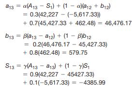
We may now update the parameters based on the observed value for period 13, A₁₃ = 42,227:  

Other calculations are similar. To forecast period 37, we use formula (9.21): 

F_{36 + 1} = a₃₆ + b₃₆(1) + S_{36 - 12 + 1} = 49,267 units 

Notice from the chart that the additive model appears to fit the data extremely well. Again, we can easily experiment with different values of the smoothing constants to find a best fit using an error measure such as MAD or MSE.

a13 a(A13 S) + (1 a)(a12 + b12). 0.3(42,227-(-5,617.33)) - +0.7(45,427.33 + 462.48) 46,476.17 b13= B(a13a12) + (1-B)b12 = = 0.2(46,476.17 - 45,427.33) +0.8(462.48) = 579.75 S13 (A13a13) + (1 - y)S = 0.9(42,227-45427.33) +0.1(-5,617.33) = -4385.99