New Semester Started Get 50% OFF Study Help! --h --m --s Claim Now

Question Answers

Textbooks

Find textbooks, questions and answers

Oops, something went wrong!

Change your search query and then try again

Result Not Found

Books FREE
Study Help
Tutors
AI Study Planner NEW
Sell Books

Search
Sign In
Register

study help
business
probability statistics

Introduction To Probability And Statistics For Science Engineering And Finance 1st Edition Walter A. Rosenkrantz - Solutions

Problem 4.44 The random variable X has a binomial distribution with parameters n = 25 and p = 0.5. (a) Compute the exact value of P(9 ≤ X ≤ 16) using the binomial tables in the text. (b) Compute P(9 ≤ X ≤ 16) using the normal approximation to the binomial. (c) Compute the same probability
Problem 4.43 Suppose the distribution of a stock price S(t) (t measured in years) is log[1]normal with parameters µ = 0.20, volatility σ = 0.30, and initial price S0 = $60. Compute: (a) E(stock price after 3 months). (b) σ(stock price after 3 months). (c) Find the probability of a loss after 3
Problem 4.42 Suppose the distribution of a stock price S(t) (t measured in years) is log[1]normal with parameters µ = 0.15, volatility σ = 0.25, and initial price S0 = $40. Compute: (a) E(stock price after 6 months). (b) σ(stock price after 6 months). (c) Find the probability of a loss after 6
Problem 4.41 Refer to Example 4.15. (a) Compute: E(ln(S(0.5), σ(ln(S(0.5)), E((S(0.5), σ(S(0.5)). (b) What is the probability that the stock’s price will be up at least 30% after six months? (c) What is the probability that the stock’s price will be down at least 20% after six months?
Problem 4.40 Suppose the combined SAT scores of students admitted to a college are normally distributed with µ = 1200 and σ = 150. Compute the value of c for which P(|X − 1200| < c)=0.5 The interval [1200 −c, 1200 + c] is the interquartile range.
Problem 4.39 Assume that math SAT scores are normally distributed with µ = 500 and σ = 100. (a) What proportion of the students have a math SAT score greater than 650? (b) What proportion of the students have a math SAT score less than 550? (c) Ten students are selected at random. What is the
Problem 4.38 Derive Equation 4.44 for the critical value x(α) of the normal distribution N(µ, σ2).
Problem 4.37 The random variable X D = N(60, 25). Compute: (a) P(X < 50) (b) P(X > 65) (c) The value of c such that P(| X − 60 |
Problem 4.36 The random variable X D = N(12, 36). (a) Compute P(X < 0), P(X > 20) (b) Find c such that: P(|X − 12| < c)=0.9, 0.95, 0.99
Problem 4.35 Suppose that a manufacturing process produces resistors whose resistance (measured in ohms) is normally distributed with µ = 0.151 and σ = 0.003. The specifications for the resistors require that the resistance equals 0.15 ± 0.005 ohms. What proportion of the resistors fail to meet
Problem 4.34 The distribution of the lifetime in hours of a battery for a laptop computer is modeled as a normal random variable with mean µ = 3.5 and standard deviation σ = 0.4 Compute the safe life of the battery, which is defined to be the 10th percentile of the distribution.
Problem 4.33 The results of a statistics exam are assumed to be normally distributed with µ = 65 and σ = 15. In order to get an A the student’s rank must be in the 90th percentile or above. Similarly, in order to get at least a B the student’s rank must be in the 80th percentile or above. (a)
Problem 4.32 Miles per gallon (mpg) is a measure of the fuel efficiency of an automobile. The mpg of a compact automobile selected at random is normally distributed with µ = 29.5 and σ = 3. (a) What proportion of the automobiles have a fuel efficiency that is greater than 24.5 mpg? (b) What
Problem 4.31 Find c such that (a) P(Zc)=0.025 (f) P(|Z|
Problem 4.30 Estimate each of the following probabilities using Chebyshev’s inequality and compare the estimates with the exact answers obtained from the tables of the normal distribution. (a) P(|Z| > 1) (b) P(|Z| > 1.5) (c) P(|Z| > 2)
Problem 4.29 Let Z be a standard normal random variable. Use the table of the normal distribution to compute the following probabilities. (a) P(Z < 1) (b) P(Z < −1) (c) P(|Z| < 1) (d) P(Z < −1.64) (e) P(Z > 1.64) (f) P(|Z| < 1.64) (g) P(Z > 2) (h) P(|Z| > 2) (i) P(|Z| < 1.96)
Problem 4.28(a) Verify by direct calculation that Q(p) = exp(− ln(1 − p)/α) − 1 is the p quantile of the Pareto distribution (Equation 4.24), that is show that F(Q(p)) = p. (b) Using part (a), compute the median of a Pareto distribution with α = 1.5.
Problem 4.27 Refer to Example 4.6. Derive the formulas for the mean and variance, given in Equation 4.24, of the random variable T with the Pareto distribution (Equation 4.24).
Problem 4.26 Suppose the lifetime T of an electronic component is exponentially dis[1]tributed with θ−1 = 1000 and the warranty period is 700 hours. The manufacturing costs and selling price of each component are $6.00 and $10.00, respectively. If the item fails before K hours the manufacturer
Problem 4.25 Let X denote a random variable with continuous df F(x) defined below. F(x)=0, x ≤ −1; F(x)=(x3/2) + 1/2, −1 ≤ x ≤ 1; F(x)=1, x ≥ 1. Compute E(X), E(X2), and V (X).
Problem 4.24 Verify Equations 4.21 and 4.22 by performing the integration by parts.
Problem 4.23 Show that if U is uniformly distributed over [0, 1] then X = a + (b − a)U is uniformly distributed over [a, b].
Problem 4.22 Let Θ be uniformly distributed over the interval [0, 2π]. Compute: (a) E(cos Θ), V (cos Θ). (b) E(sin Θ), V (sin Θ). (c) E(| cos Θ|). (d) Does E(cos Θ) = cos (E(Θ))?
Problem 4.21 If X is uniformly distributed over the interval [a, b] show that: (a) E(X)=(a + b)/2. (b) V (X)=(b − a)2/12.
Problem 4.20 Let S denote the random variable described in Problem 4.12. Compute: (a) E(S) (b) V (S)
Problem 4.19 Compute E(X), E(X2), and V (X) for the random variable X with pdf given by: (a) f(x) = 1 2 − x 4 , −1 ≤ x ≤ 1, f(x)=0, elsewhere. (b) f(x) = (1/2) sin x, 0 ≤ x ≤ π, f(x)=0, elsewhere. (c) f(x) = 3(1 − x) 2, 0
Problem 4.18 Consider the random variable X with distribution function F(x)=0, x ≤ 0, F(x)=1 − 1 (1 + x)2 ,x> 0. (a) Graph F(x) for all x. (b) Compute the pdf f(x) for all x and sketch its graph. (c) Compute P(1
Problem 4.17 Which of the following functions F(x) are continuous dfs of the form dis[1]played in Definition 4.1? Calculate the corresponding pdf f(x) where appropriate. (a) F(x)=0, x ≤ 0, F(x) = x 1 + x ,x> 0; (b) F(x)=0, x ≤ 2, F(x)=1 − 4 x2 ,x> 2; (c) F(x)=0,x< −π/2, F(x) = sin x,
Problem 4.16 Let X denote a random variable with continuous df F(x) defined below. F(x)=0, x ≤ −1, F(x)=(x3/2) + 1/2, −1 ≤ x ≤ 1, F(x)=1, x ≥ 1. (a) Graph F(x) for all x. (b) Compute the pdf f(x) for all x and sketch its graph. (c) Compute the 10th and 90th percentiles of the
Problem 4.15 Suppose the number of days to failure of a diesel locomotive has an ex[1]ponential distribution with parameter 1/θ = 43.3 days. Compute the probability that the locomotive operates one entire day without failure.
Problem 4.14 Refer to the lifetime distribution in Problem 4.13. Compute the safe life of the diesel engine fan. (The safe life of a component is the 10th percentile of its lifetime distribution; it is the length of time that 90% of the components will operate without failure.)
Problem 4.13 Suppose the lifetime of a fan on a diesel engine has an exponential distri[1]bution with 1/θ = 28, 700 hours. Compute the probability of a fan failing on a: (a) 5, 000 hour warranty. (b) 8, 000 hour warranty.
Problem 4.12 The thickness S (measured in millimeters) of a fiber thread has a pdf given by f(x) = kx2(2 − x), 0 1).
Problem 4.11 The lifetime T (in hours) of a component has a df given by F(t)=0, t ≤ 1, F(t)=1 − 1 t2 , t ≥ 1. (a) Sketch the graph of F(t). (b) Compute the pdf f(t) of T and sketch its graph. (c) Find P(T > 100). (d) Compute P(T > 150|T > 100), i.e., given that the component is still
Problem 4.10 The random variable X has pdf given by f(x) = (1 + x), −1 ≤ x ≤ 0, f(x) = (1 − x), 0 ≤ x ≤ 1, f(x)=0, elsewhere. (a) Sketch the graph of f(x). (b) Compute the df F(x) for all values of x and sketch its graph. (c) Compute P(−0.4
Problem 4.9 An archer shoots an arrow at a circular target. Suppose the distance between the center and impact point of the arrow is a continuous random variable X(meters) with pdf given by f(x)=6x(1 − x), 0
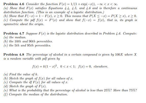
Problem 4.8 The percentage of alcohol in a certain compound is given by 100X where X is a random variable with pdf given by f(x)=k(1-x)2, 0
Problem 4.6. Compute: (a) the median. (b) the 10th and 90th percentiles. (c) the 5th and 95th percentiles.
Problem 4.7 Suppose F(x) is the logistic distribution described in
Problem 4.6 Consider the function F(x)=1/(1+ exp(-2)), - < 1
Problem 4.3 Let Y denote a random variable with continuous df F(y) defined below. F(y)=0, y ≤ 0, F(y) = y3/8, 0 < y ≤ 2, F(y)=1,y > 2. (a) Graph F(y) for all y. (b) Compute P(0.2 0.6). (c) Compute the pdf f(y) for all y and sketch its graph. Problem 4.6 Consider the function F(x) = 1/(1+
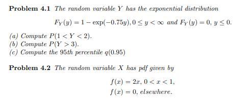
Problem 4.2 The random variable X has pdf given by f(x)=2r, 0 <
Problem 4.1 The random variable Y has the exponential distribution Fy (y) 1 exp(-0.75y), 0 < y < and Fy (y) = 0, y 0. (a) Compute P(1 < < 2). (b) Compute P(Y > 3). (c) Compute the 95th percentile q(0.95)
Problem 3.77(a) Derive the formula for the mgf of the geometric distribution displayed Equation 3.70. (b) Use the mgf to compute the first two moments and the variance of the geometric distri[1]bution. Problem 4.1 The random variable Y has the exponential distribution Fy (y) 1-exp(-0.75y), 0 < y <
Problem 3.76(a) Derive the formula for the mgf of the Poisson distribution displayed in Equation 3.69. (b) Use the mgf to compute the first two moments and the variance of the Poisson distri[1]bution.
Problem 3.75 A sampling plan has n = 100, c = 2 and the lot size N=10,000. Compute the approximate acceptance probabilities for the following values of D: (a) D = 50 (b) D = 100 (c) D = 200 Hint: Use the Poisson approximation to the binomial.
Problem 3.74 A taxi company has a limousine with a seating capacity of N. The cost of each seat is $5 and the price per seat is $10. The number of reservations X is Poisson distributed with parameter λ = 5, i.e., P(X = x) = e−55x/x!, x = 0, 1 ....Compute the expected net revenue when: (a) N = 4
Problem 3.73 A computer disk drive is warranted to last at least 4,000 hours. The prob[1]ability that a disk drive lasts 4,000 or more hours equals 0.9999. (a) Let X denote the number of disk drive failures during the warranty period. Describe the distribution of X; name it and identify the
Problem 3.72 A batch of dough yields 500 cookies. How many chocolate chips should be mixed into the dough so that the probability of a cookie having no chocolate chips is ≤ .01?
Problem 3.71 The number of chocolate chips per cookie is assumed to have a Poisson distribution with λ = 4. Find the probability that: (a) a cookie has no chocolate chips. (b) a cookie has 7, or more, chocolate chips.
Problem 3.70 The prevalence rate for a rare disease is 3 per 10,000. (a) Let X denote the number of cases (of the disease) in a small town of population 8, 000. Describe the exact distribution of X; name it and identify the parameters. (b) What is the expected number of town residents with the
students?
Problem 3.69 If 99% of students entering a junior high school are vaccinated against the measles, what is the probability that a group of 50 students contain: (a) no unvaccinated students? (b) exactly one unvaccinated student? (c) two or more unvaccinated
Problem 3.68 A lot of 10, 000 articles has 150 defective items. A random sample of 100 articles is selected. Let X denote the number of defective items in the sample. Give the formula for: (a) the exact pf fX(x) of X. (b) the binomial approximation of fX(x). (c) the Poisson approximation of the
Problem 3.67(a) Compute the Poisson probabilities p(x; 1.5), x = 0, 1, 2, 3 using Equa[1]tion 3.60. (b) Compute the Poisson probabilities p(x; 1.5), x = 0, 1, 2, 3 using the formula p(x; λ) = P(x; λ) − P(x − 1; λ), where the values of the distribution function P(x; λ) = 0≤y≤x p(y; λ)
Problem 3.66(a) Compute p(x; 2), x = 0, 1, 2, 3 using Equation 3.60. (b) Compute p(x; 2), x = 0, 1, 2, 3 using the recurrence relation 3.63.
Problem 3.65 Verify Equation 3.62.
Problem 3.64 The random variable X has a binomial distribution with parameters n = 20 and p = 0.01. In each of the following cases compute: (i) the exact value of P(X = x) and (ii) its Poisson approximation for: (a) x = 0; (b) x = 1; (c) x = 2.
Problem 3.63 The probability that a disk drive lasts 6000 or more hours equals 0.8. In a batch of 20, 000 disk drives how many would be expected to last 6000 or more hours?
Problem 3.62 Can Chebyshev’s inequality be improved? Consider the random variable X with the following probability function: P(X = ±a) = p, P(X = 0) = 1 − 2p, (0)
Problem 3.61 R. Wolf (1882) threw a die 20, 000 times and recorded the number of times each of the six faces appeared. The results follow. Face 123456 Frequency 3407 3631 3176 2916 3448 3422 (Source: D. J. Hand, et. al. (1994), Small Data Sets, Chapman& Hall, London.) (a) Compute an upper bound on
Problem 3.60 Verify that choosing the parameters of the binomial lattice model as in Equation 3.54 yields the values for the mean and variance given in Equation 3.55.
Problem 3.59 Compute the expected value and standard deviation (risk) of the return (after one month) on the stock described in Problem 3.58.
Problem 3.58 Assume the price moves of a stock follows the binomial lattice model de[1]scribed in Example 3.25 with initial price S0 = $75 and parameters u = 1.015, d = 0.985, p = 0.52. Assume the time period is one week. (a) Give the formula for the probability distribution S4, which is the stock
Problem 3.57 Compute the expected value and standard deviation (risk) of the return (after one month) on the stock described in Problem 3.56.
Problem 3.56 Assume the price moves of a stock follows the binomial lattice model de[1]scribed in Example 3.25 with initial price S0 = $50 and parameters u = 1.02, d = 0.99, p = 0.52. Assume the time period is one week. (a) Give the formula for the probability distribution S4, which is the stock
Problem 3.55 Suppose X is a random variable with µX = 50, σX = 4. Using only this information show that P(42 ≤ X ≤ 58) ≥ 0.75.
Problem 3.54 Suppose X is a random variable with µX = 20, σX = 1. Using only this information show that P(|X − 20| ≥ 4) ≤ 0.0625.
Problem 3.53 Let X denote the number of heads in n tosses of a fair coin. Use Cheby[1]shev’s inequality to obtain a lower bound on the following probabilities: (a) P(225 ≤ X ≤ 275) when n = 500. (b) P(80 ≤ X ≤ 120) when n = 200. (c) P(45 ≤ X ≤ 55) when n = 100.
Problem 3.52 Use Chebyshev’s inequality to estimate the probability that the sample pro[1]portion obtained from a poll of voters with a sample size of n = 2500 differs from the true proportion by an amount less than or equal to 0.04.
Problem 3.51(Continuation of Problem 3.50) Suppose 200 patients are given the drug. Let R denote the number of patients who recover. Compute E(R) and V (R) for each of the following two cases: (a) the drug is worthless. (b) the drug is really 80% effective as claimed.
Problem 3.50 It is known that 40% of patients naturally recover from a disease. A drug is claimed to cure 80% of all patients with the disease. An experimental group of 20 patients is given the drug. What is the probability that at least 12 recover if: (a) The drug is worthless and hence the true
Problem 3.49 A sampling plan has n = 20 and the lot size N = 1, 000. (a) Compute the acceptance probabilities for D = 50 acceptance number c = 2. Hint: Use the binomial approximation to the hypergeometric distribution. (b) Compute the acceptance probabilities for D = 50 and acceptance number c = 1.
Problem 3.48 The lifetime (measured in hours) of a randomly selected battery is a random variable denoted by T . Assume that P(T ≤ 3.5) = 0.10. This means that 90% of the batteries have lifetimes that exceed 3.5 hours. A random sample of 20 batteries is selected for testing. (a) Let Y = the
Problem 3.47 A taxi company has a limousine with a seating capacity of N. The main[1]tenance cost (to the taxi company) of each seat is $5, and the price per seat is $10. The number of reservations is a binomial random variable X with parameters n = 10, p = 0.4. Compute the expected net revenue
Problem 3.46 Let Y denote the number of times a 1 appears in 720 throws of a die. Compute E(Y ) and V (Y ).
Problem 3.41 The random variable X has the binomial distribution B(x; n, p). Compute the following probabilities using the binomial tables. (a) P(X ≤ 4) = B(4; 10, p) for p = 0.1, 0.4, 0.6, 0.8 (b) P(X > 9) = 1 − B(9; 20, p) for p = 0.2, 0.5, 0.7, 0.9 Problem 3.42 For n = 20 and p = 0.5 (a)
Problem 3.40 Compute each of the following binomial probabilities in two ways: (1) by using Equation 3.33, and (2) by using the Equation 3.40 together with the binomial tables in Appendix A. (a) b(0; 20; 0.1), b(1; 20; 0.1), b(5; 20; 0.1) (b) b(2; 10; 0.4), b(4; 10; 0.4), b(7; 10; 0.4)
Problem 3.39 An urn contains two white balls and four red balls. Balls are drawn one by one without replacement until two white balls have appeared. Denote by U the number of balls that must be drawn until both white balls have appeared. Compute the pf of U.
Problem 3.38 An urn contains 2 nickels and 3 dimes.We select two coins at random,without replacement. Let X= monetary value of the coins in the sample,e.g., if the sample consists of a nickel and dime then X=15 cents. (a) Compute the pf of X. (b) Compute E(X). (c) Compute V(X).
Problem 3.37 A group of 10 items contains 2 that are defective. Articles are taken one at a time from the lot and are tested. Let Y denote the number of articles tested in order to find the first defective item. Compute the pf of Y.
Problem 3.36 Suppose a sample of size 15 is taken from a lot of 50 items and the lot is accepted if the number X of defective items in the sample is less than or equal to one, i.e., we accept the lot if X ≤ 1. Compute the P(acceptance) for the following values of D: (a) D = 1 (b) D = 3 (c) D = 6
Problem 3.35 Suppose the sampling plan is to sample 10% of a lot of N items and the acceptance number c = 0. Compute the acceptance probability in each of the following cases: (a) N = 50, D = 1 (b) N = 100, D = 2 (c) N = 200, D = 4
Problem 3.34 A lot of 10 components contains 2 that are defective. A random sample of size 4 is drawn. Let X denote the number of defective components that are drawn. (a) Show that X has a hypergeometric distribution and identify the parameters N, D, n. Use the formula from part (a) to compute the
Problem 3.33 The random variable X has a hypergeometric distribution with parameters n = 4, N = 20, D = 6. (a) Compute h(x), x = 0, 1, 2, 3, 4 using Equation 3.28. (b) Compute h(x), x = 0, 1, 2, 3, 4 using the recurrence Equation 3.31. Which method is the more efficient for computing the
Problem 3.32 The random variable X has the discrete uniform distribution (see Equation 3.16). Show that V (X) = (N − 1)(N + 1) 12 . Hint: Use the shortcut formula and Equation 3.15 for the moments of the discrete uniform distribution.
Problem 3.31 Let X be a Bernoulli random variable. Show that V (X) ≤ 1 4 . Hint: The variance of a Bernoulli random variable is given by V (X) = p(1 − p) (see Equation 3.22). Then show that p(1 − p) ≤ 1/4.
Problem 3.30 The random variable X has the pf defined by f(x) = 1 x(x + 1) for x = 1, 2, . . . , n, . . . . Show that E(X) = ∞ by verifying that 1≤x
Problem 3.29 Let X have the pf given by: f(x) = 2x n(n + 1) for x = 1, 2,...n; f(x)=0 elsewhere. Compute E(X). Hint: Use Equation 3.17.
Problem 3.28 Compute E(W) and V (W) for the random variable W of Problem 3.7.
Problem 3.27 The random variable X has the pf defined by f(x) = (6 − x)/30 for x = −2, −1, 0, 1, 2; f(x)=0 elsewhere. Compute: (a) E(X) (b) E(X2) (c) V (X) (d) E(2X) (e) E(2−X) (f) E(cos(πX))
Problem 3.26 Let the random variable Y have the distribution function F(y) defined by: F(y)=0,y < −1 F(y)=0.2, −1 ≤ y < 0 F(y)=0.5, 0 ≤ y < 1 F(y)=0.8, 1 ≤ y < 3 F(y)=1, y ≥ 3 Compute: (a) E(Y ) (b) E(Y 2) (c) V (Y )
Problem 3.25 The random variable X has the pf defined by f(x) = 5−x2 15 ; x = −2, −1, 0, 1, 2; f(x)=0 elsewhere. Compute: (a) E(X) (b) E(X2) (c) V (X) (d) E(2X) (e) E(2−X) (f) E(cos(πX)).
Problem 3.24 The random variable X has pf given by the following table: x −2 −1 0 1 2 f(x) 0.2 0.1 0.1 0.4 0.2 Compute: (a) E(X) (b) E(X2) (c) V (X) (d) E(2X) (e) E(2−X) (f) E(sin(πX))
Problem 3.23 Suppose E(X)=2, E(X2)=6, E(X3) = 22 . Compute: (a) V (X) (b) E((X − 1)2) (c) E((X − 1)3)
Problem 3.22 Suppose E(X)=2, V (X)=9. Compute: (a) E(3X − 6) (b) E(X2) (c) E(X + 1)2
Problem 3.21 The random variable X has pf defined by: f(x) = 1 5 ; x = 1, 2, 3, 4, 5; f(x)=0 elsewhere. Compute: (a) E(X) (b) E(X2) (c) V (X) (d) E(2X) (e) E( √ X) (f) E(2X + 5) (g) V (2X + 5)
Problem 3.20 The payoff of a one-roll bet on the number 11 is 15 to 1. (a) Compute the house percentage. Note: The definition of house percentage is given in Definition 3.6. (b) Compute the true odds. For the definition of true odds refer to Equation 3.11.
Problem 3.19 Compute E(X) and V (X) where X is the number of hearts inafive-card poker hand. Hint: Use Equation 3.4 to compute fX(x).
Problem 3.18 Table 3.3 displays the probability function corresponding to the experiment of throwing two dice. Compute E(X) and V (X).

Showing 6800 - 6900 of 8686

First
62
63
64
65
66
67
68
69
70
71
72
73
74
75
76
Last

Step by Step Answers

Services

Sitemap
Fun
Definitions
Become Tutor
Used Textbooks
Study Help Categories
Recent Questions
Expert Questions
Campus Wear
Sell Your Books

Company Info

Security
Copyrights
Privacy Policy
Terms & Conditions
SolutionInn Fee
Scholarship
Online Quiz
Give Feedback, Get Rewards

Get In Touch

About Us
Contact Us
Career
Jobs
FAQ
Student Discount
Campus Ambassador

Secure Payment

Download Our App

© 2026 SolutionInn. All Rights Reserved