New Semester
Started
Get
50% OFF
Study Help!
--h --m --s
Claim Now
Question Answers
Textbooks
Find textbooks, questions and answers
Oops, something went wrong!
Change your search query and then try again
S
Books
FREE
Study Help
Expert Questions
Accounting
General Management
Mathematics
Finance
Organizational Behaviour
Law
Physics
Operating System
Management Leadership
Sociology
Programming
Marketing
Database
Computer Network
Economics
Textbooks Solutions
Accounting
Managerial Accounting
Management Leadership
Cost Accounting
Statistics
Business Law
Corporate Finance
Finance
Economics
Auditing
Tutors
Online Tutors
Find a Tutor
Hire a Tutor
Become a Tutor
AI Tutor
AI Study Planner
NEW
Sell Books
Search
Search
Sign In
Register
study help
business
statistics econometrics
Social Statistics For A Diverse Society 9th Edition Chava Frankfort Nachmias, Anna Y Leon Guerrero, Georgiann Davis - Solutions
2. Calculate and interpret confidence intervals for means.
1. Explain the concept of estimation, point estimates, confidence level, and confidence interval.
C7. From the GSS 2018 subsample, we find that 83% of respondents believe in life after death (N = 1,054).1. What is the 95% confidence interval for the percentage of the U.S. population who believe in life after death?2. Without doing any calculations, estimate the lower and upper bounds of 90% and
C8. A social service agency plans to conduct a survey to determine the mean income of its clients. The director of the agency prefers that you measure the mean income very accurately, to within ±$500. From a sample taken 2 years ago, you estimate that the standard deviation of income for this
E1. Investigate whether or not Americans have 12 years of education.1. Perform a one-sample t test with the variable EDUC (highest year of school completed). See Excel Demonstration 1 as an example.2. What is the mean value of EDUC?3. What is the obtained t value?4. What is the p value for a
E2. Compare the mean years of education (EDUC) by sex. Do females complete more years of education than males?1. Test the mean difference of EDUC (highest year of school completed) by SEX (respondent’s sex). See Excel Demonstration 2 as an example.2. What is the mean value of EDUC for females?
C1. It is known that, nationally, doctors working for health maintenance organizations(HMOs) average 13.5 years of experience in their specialties, with a standard deviation of 7.6 years. The executive director of an HMO in a western state is interested in determining whether or not its doctors
C2. In this chapter, we examined the difference in educational attainment between firstand second-generation Hispanic and Asian Americans based on the proportion of each group with a bachelor’s degree. We present additional data from the Pew Research Center’s 2013 report, measuring the
C3. For each of the following situations, determine whether a one- or a two-tailed test is appropriate. Also, state the research and the null hypotheses.1. You are interested in finding out if the average household income of residents in your state is different from the national average household.
C4. In 2016, the Pew Research Center16 surveyed 1,799 white and 1,001 black Americans about their views on race and inequality. Pew researchers found “profound differences between black and white adults in their views on racial discrimination, barriers to black progress and the prospects for
C5. One way to check on how representative a survey is of the population from which it was drawn is to compare various characteristics of the sample with the population characteristics. A typical variable used for this purpose is age. The GSS 2018 found a mean age of 48.69 and a standard deviation
E2. Is there a significant difference in the age at which a respondent’s first child was born(AGEKDBRN) among different educational groups (DEGREE)?1. Run an ANOVA test of AGEKDBRN by DEGREE.2. What is the value of the F statistic? What p value is associated with this F statistic?3. Is there a
E1. Investigate whether there is a significant difference in the number of ideal children (CHLDIDEL)by marital status (MARITAL).1. Run an ANOVA test of CHLDIDEL by MARITAL.2. What is the mean ideal number of children for married respondents? Widowed? Divorced?Separated? Never married?3. What is the
S5. Repeat Exercise S4, separating results by SEX. Does the relationship change when including SEX as a control variable? Explain.
S4. Using GSS18SSDS-B, treat NEWS (how often do you read the newspaper) as your dependent variable and DEGREE (respondent’s educational degree) as your independent variable. Setting alpha = .05, assess the significance of both models. NEWS is coded on a 5-point scale: 1 =everyday, 2 = few times a
S3. What is the ideal number of children a family should have (variable CHLDIDEL)? Use CHLDIDEL as your dependent variable and DEGREE as your independent variable. Is there a significant difference in the number of ideal children among different educational groups? (Option:You can run three sets of
S2. Repeat Exercise 1b, substituting respondent’s social class (CLASS) as the independent variable in separate models for men and women. What can you conclude about the relationship between CLASS and AGEKDBRN based on an alpha of .01?
S1. Let’s continue to examine the relationship between fertility decisions and education using GSS18SSDS-A. But this time, we’ll analyze the relationship for men.1. Run a Select Cases, selecting only men for the analysis.2. Compute an ANOVA model for men, using age at first-born child
For the “Sense of Belonging and Satisfaction” ANOVA model, what additional information would you need to determine the F critical?
If alpha were changed to .01, would our final decision change?
5. How to Interpret output for ANOVA.
4. Determine the significance of an F-ratio test statistic.
3. Calculate and interpret a test for two or more sample cases with means.
2. Define the concepts of between and within total variance.
1. Explain the application of a one-way analysis of variance (ANOVA) model.
C6. According to the GSS 2018, 51% of 218 college graduates reported being interested in environmental issues compared with 43% of 167 high school graduates.1. What is the research hypothesis? Should you conduct a one- or a two-tailed test?Why?2. Present the five-step model, testing your hypothesis
C7. GSS 2018 respondents were asked to rate their level of agreement to the statement,“Differences in income in America are too large.” Responses were measured on a 5-point scale: 1 = strongly agree, 2 = agree, 3 = neutral, 4 = disagree, and 5 = strongly disagree.Strong Democrats had an average
C8. We compare the proportion who indicated speaking a language other than English for two GSS 2018 groups: respondents (1) born in the United States (native born) and (2) not born in the United States (foreign born). Test the research hypothesis that a lower proportion of native-born respondents
C9.In surveys conducted during August 2016 (months before the election), the Pew Research Center reported that among 752 men, 55% indicated that regardless of how they felt about Hillary Clinton, the election of a woman as president would be very important historically. Among 815 women, 65%
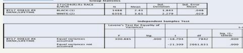
C10. In this SPSS output, we examine lifetime use of alcohol among white and black students based on the MTF 2017. Lifetime use is measured on an ordinal scale: 1 = 0 occasions, 2 = 1–2 times, 3 = 3–5 times, 4 = 6–9 times, 5 = 10–19 times, 6 = 20–39 times, and 7 = 40+. Present Step 5
If alpha was changed to .01, one-tailed test, would your final decision change?Explain.
State the null and research hypothesis for this SPSS example. Would you change your decision in the previous example if alpha was .01? Why or why not?
C10.Th roughout the 2016 presidential election primaries, Millennials (those aged 20 to 36 years)consistently supported Senator Bernie Sanders over Secretary Hillary Clinton. According to the 2016 Gallup poll of 1,754 Millennials, 55% had a favorable opinion of Sanders compared with Hillary Clinton
C12. According to a report published by the Pew Research Center in February 2010, 61%of Millennials (Americans in their teens and 20s) think that their generation has a unique and distinctive identity (N = 527).18 1. Calculate the 95% confidence interval to estimate the percentage of Millennials
C13. In 2018, GSS respondents (N = 1,117) were asked about their political views. The data show that 29% identified as liberal, while 32% were identified as conservative.1. For each reported percentage, calculate the 95% confidence interval.2. Approximately 39% of GSS respondents identified as
E3. Does a respondent’s preferred candidate in the 2016 presidential election (PRES16) vary by political views (RE_POLVIEWS)? Treat RE_POLVIEWS as the independent variable and PRES16 as the dependent variable.1. Create a bivariate table of observed frequencies for RE_POLVIEWS and PRES16.2. Create
E2. Do political views (RE_POLVIEWS) vary by marital status (MARITAL)? Treat MARITAL as the independent variable and RE_POLVIEWS as the dependent variable.1. Create a bivariate table of observed frequencies for MARITAL and RE_POLVIEWS.2. Create a bivariate table of expected frequencies for MARITAL
E1. Do attitudes toward premarital sex (PREMARSX) vary by respondent’s sex (SEX)? Treat SEX as the independent variable and PREMARSX as the dependent variable.1. Create a bivariate table of observed frequencies for SEX and PREMARSX.2. Create a bivariate table of expected frequencies for SEX and
For the bivariate table with age and first-generation college status (first presented in Learning Check 10.1), the value of the obtained chi-square is 181.15 with 1 degree of freedom. Based on Appendix D, we determine that its probability is less than .001.This probability is less than our alpha
What decision can you make about the association between age and firstgeneration college status? Should you reject the null hypothesis at the .05 alpha level or at the.01 level?
Refer to the data in Learning Check 10.1. Calculate the expected frequencies for age and first-generation college status and construct a bivariate table. Are your column and row marginals the same as in the original table?
1. Describe the assumptions of statistical hypothesis testing.
Refer to the data in the previous Learning Check. Are the variables age and first-generation college status statistically independent? Write out the research and the null hypotheses for your practice data
6. Interpret output for chi-square and measures of association.
5. Apply and interpret measures of association: lambda, Cramer’s V, gamma, and Kendall’s tau-b.
2. Define and apply the components in hypothesis testing.
4. Explain the concept of proportional reduction of error.
3. Determine the significance of a chi-square test statistic.
2. Calculate and interpret a test for the bivariate relationship between nominal or ordinal variables.
1. Summarize the application of a chi-square test.
3. Explain what it means to reject or fail to reject a null hypothesis.
C13. In Exercise 5, we presented MTF 2017 data for all 12th graders. In this exercise, we present the same data but only for the 1,460 respondents who identified as males.Ca lcu lat e the percentages using race as the independent variable. Is there a relationship for males between race and their
C12. The following table draws on GSS18SSDS-B data so we can examine the relationship between citizenship status and satisfaction with financial situation.1. Identify the independent variable, dependent variable, and control variable.2. How many total people are included in the table? How many are
C11. Let’s continue our examination of variation in household division of labor from Exercise 7 by focusing on men. The following table has been adapted from Tsui-o Tai and Janeen Baxter’s (2018) analysis to show the relationship between perceived unfairness and frequency of housework
4. Calculate and interpret a test for two sample cases with means or proportions.
C10. In the 2013 ISSP, respondents in several European countries were asked their level of agreement to the statement, “Immigrants take jobs away from people born in their country.” Their responses (frequencies only) are presented below.1. Is th er ea relationship between a respondent’s
C9. Daniel Rocke and his colleagues (2014) assessed support of the Patient Protection and Affordable Care Act among a sample of 647 otolaryngology (ear, nose, and throat)physicians. They divided physicians by political party affiliation—Democrat, Other, and Republican (refer to the following
C8. In Exercise 1, you found that more women than men are likely to fear walking alone in their neighborhoods. You now wonder if this difference exists because women are more likely to own their own homes and therefore live in safer neighborhoods. In other words, you want to try some elaboration.1.
C7. Drawing on International Social Survey Programme data, Tsui-o Tai and Janeen Baxter (2018) examined variation in household division of labor. The following table has been adapted from their analysis to show the relationship between perceived unfairness and frequency of housework disagreement
5. Determine the significance of t-test and Z-test statistics.
C6. The following cross-tabulation, based on GSS18SSDS-B data, examines the relationship between age (the independent variable) and whether or not one feels discriminated against because of age. As with Exercise 2, we have recoded age into four categories: 18–29, 30–39, 40–49, and 50–59.
C5. Youth were asked in the Monitoring the Future (MTF) 2017 survey to report how often they were drunk in the past 12 months. Responses for 3,176 twelfth graders are reported by race.Ca lcu lat ethe percentages using race as the independent variable. Is there a relationship between race and
C4. We continue our examination of attitudes regarding home ownership. Suppose that a classmate of yours suggests that home ownership can be explained by age. Your classmate shows you the following table taken from the GSS18SSDS-B sample.(Frequencies are shown below.)is the dependent variable in
C3. One of your classmates hypothesizes that people of color are far less likely to own their own home than white people. Use the following data, which draws from GSS18SSDS-B, to test your classmate’s hypothesis.your classmate’s argument, what is the dependent variable? The independent
C2. The following cross-tabulation, based on GSS18SSDS-B data, examines the relationship between age (the independent variable) and presidential candidate one voted for in the 2016 U.S. presidential election (dependent variable). Notice we have recoded age into four categories: 18–29, 30–39,
The implications of research findings are not created equal. For example, researchers might hypothesize that eating spinach increases the strength of weightlifters. Little harm will be done if the null hypothesis that eating spinach has no effect on the strength of weightlifters is rejected in
E3. Does the relationship between marital status (MARITAL) and social class (CLASS) vary by respondent’s sex (SEX)?1. Use Excel’s PivotTable command to create a bivariate table of the relationship between MARITAL and CLASS for all respondents, male respondents, and female respondents. Treat
E2. Is there a relationship between one’s sexual orientation (SEXORNT) and their political views(RE_POLVIEWS)?1. Use Excel’s PivotTable command to create a bivariate table of SEXORNT (independent variable) and RE_POLVIEWS (dependent variable).2. What percentage of all respondents identified as
E1. Investigate the relationship between respondent’s sex (SEX) and highest degree earned(DEGREE).1. Use Excel’s PivotTable command to create a bivariate table of SEX (independent variable) and DEGREE (dependent variable).2. What percentage of all respondents reported a high school diploma as
S5. Let’s examine the relationship between subjective class identification (CLASS) and confidence in medicine (CONMEDIC). Define CONMEDIC as the dependent variable.1. Is there a relationship between CLASS and CONMEDIC? Explain your answer using percentages from the cross-tabulations you’ve
S4. In this exercise, test the relationship between subjective class identification (CLASS) and feelings about government spending on the following social issues: crime rate (NATCRIME), educational system (NATEDUC), and nation’s health (NATHEAL). You will produce a total of three
S3. Let’s further examine which candidate respondents voted for in the 2016 presidential election(PRES16). Examine the relationship between PRES16, GETAHEAD (opinion of how people get ahead), and SEX. Treat PRES16 as the dependent variable, GETAHEAD as the independent variable, and SEX as the
S2. We continue to explore attitudes toward homosexuality, this time using SEX (respondent’s sex)as an independent variable rather than as a control variable as we did in SPSS Demonstration 2.Use SPSS to construct a table showing the relationship between SEX (independent variable) and HOMOSEX
S1. Is there a relationship between a respondent’s subjective class identification (CLASS) and the candidate they voted for the in the 2016 U.S. presidential election (PRES16)? To answer this question, use the SPSS Crosstabs procedure, requesting counts and appropriate cell percentages.(Click on
As indicated in Table 9.5, there were a total of 11,123 people in the ELS data set sociologist Merolla relied on to conduct his study. More specifically, 15.79% of the sample was black, 17.66% was Hispanic, and 66.55% was white. How many black, Hispanic, and white people were in Merolla’s study?
Practice constructing a bivariate table. Use Table 9.1 to create a percentage bivariate table. Compare your table with Table 9.3. Did you remember all the parts? Are your calculations correct? If not, go back and review this section. It might be helpful to examine A Closer Look 9.1 below. It
Examine Table 9.2. Make sure you can identify all the parts just described and that you understand how the numbers were obtained. Can you identify the independent and dependent variables in the table? You will need to know this to convert the frequencies to percentages.
Identify the independent and dependent variables in Examples 2 and 3.
3. Explain how to elaborate the relationship between variables: nonspuriousness, intervening, and conditional relationships
2. Identify the properties of a bivariate relationship: existence, strength, and direction.
1. Create and analyze a bivariate table.
C12. The following table presents the number of parolees (per 100,000 people) for 12 of the most populous states as of July 2015.Source: National Institute of Corrections, Correction Statistics by State, 2016.1. Assume that σ = 226.83 for the entire population of 50 states. Calculate and interpret
C11. A small population of N = 10 has values of 4, 7, 2, 11, 5, 3, 4, 6, 10, and 1.1. Calculate the mean and standard deviation for the population.2. Take 10 simple random samples of size 3, and calculate the mean for each.3. Calculate the mean and standard deviation of all these sample means. How
C10. Imagine that you are working with a total population of 21,473 respondents. You assign each respondent a value from 0 to 21,473 and proceed to select your sample using the random number table in Appendix A. Starting at column 7, line 1 in Appendix A and going down, which are the first five
C9. You’ve been asked to determine the percentage of students at your university who support open border policies that would allow folks to freely move between international jurisdictions with minimal or no restrictions. You want to take a sample of 10% of the students enrolled on your campus to
C8. The following table shows the number of active military personnel in 2009, by region(including the District of Columbia).Source: U.S. Census Bureau, Statistical Abstract of the United States: 2012, Table 508 (data) and U.S. Census Bureau, Census Regions and Divisions of the United States
C7. Facebook now allows users to create a poll of their own to assess their FB friends’views on any given issue. For example, you could create a Facebook poll today asking your FB friends if they feel police brutality is a serious issue offering the response options“Yes,” “No,” and “Not
C6. When taking a random sample from a very large population, how does the standard error of the mean change when 1. the sample size is increased from 100 to 1,600?2. the sample size is decreased from 300 to 150?3. the sample size is multiplied by 4?
C3. The following four common situation scenarios involve selecting a sample and understanding how a sample relates to a population.1. A friend interviews every 10th shopper who passes by her as she stands outside one entrance of a major department store in a shopping mall. What type of sample is
C2. The mayor of your city has been talking about the need for a tax hike. The city’s newspaper uses letters sent to the editor to judge public opinion about this possible hike, reporting on their results in an article.1. Do you think that these letters represent a random sample? Why or why
C1. Explain which of the following is a statistic and which is a parameter.1. The mean age of Americans from the 2020 decennial census 2. The unemployment rate for the population of U.S. adults, estimated by the government from a large sample 3. The percentage of students at your school who receive
Suppose a population distribution has a mean μ = 150 and a standard deviation s = 30, and you draw a simple random sample of N = 100 cases. What is the probability that the mean is between 147 and 153? What is the probability that the sample mean exceeds 153? Would you be surprised to find a mean
What is a normal population distribution? If you can’t answer this question, go back to Chapter 5. You must understand the concept of a normal distribution before you can understand the techniques involved in inferential statistics.
Can you think of some research questions that could best be studied using a disproportionate stratified random sample? When might it be important to use a proportionate stratified random sample?
How does a systematic random sample differ from a simple random sample?
What is the probability of drawing an ace out of a normal deck of 52 playing cards? It’s not 1/52. There are four aces, so the probability is 4/52 or 1/13. The proportion is.08. The probability of drawing the specific ace, like the ace of spades, is 1/52 or .02.
5. Describe the central limit theorem.
4. Apply the concept of the sampling distribution.
3. Identify and apply different sampling designs.
2. Explain the relationship between a sample and a population.
Showing 7100 - 7200
of 7357
First
60
61
62
63
64
65
66
67
68
69
70
71
72
73
74
Step by Step Answers