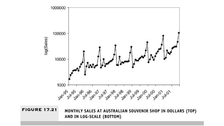
Figure 17.21 shows a time plot of monthly sales for a souvenir shop at a beach resort town in Queensland, Australia, between 1995-2001 (data are available in SouvenirSales.xls, source: Hyndman, R.J. Time Series Data Library, http://data.is/TSDLdemo, accessed on 07/25/15). The series is presented twice, in Australian dollars and in log-scale. Back in 2001, the store wanted to use the data to forecast sales for the next 12 months (year 2002). They hired an analyst to generate forecasts. The analyst first partitioned the data into training and validation sets, with the validation set containing the last 12 months of data (year 2001). She then fit a regression model to sales, using the training set.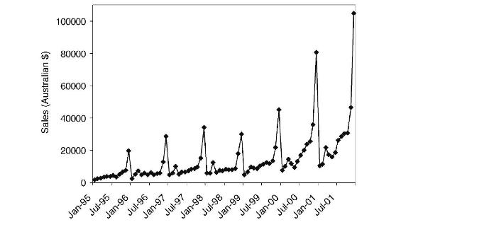

a. Based on the two time plots, which predictors should be included in the regression model? What is the total number of predictors in the model?

b. Run a regression model with Sales (in Australian dollars) as the output variable, and with a linear trend and monthly predictors. Remember to fit only the training data. Call this model A.
i. Examine the estimated coefficients. Which month tends to have the highest average sales during the year? Why is this reasonable?
ii. The estimated trend coefficient is 245.36 . What does this mean?

c. Run a regression model with \(\log (\) Sales) as the output variable, and with a linear trend and monthly predictors. Remember to fit only the training data. Call this model B.
i. Fitting a model to \(\log (\) Sales) with a linear trend is equivalent to fitting a model to Sales (in dollars) with what type of trend?
ii. The estimated trend coefficient is 0.02 . What does this mean?
iii. Use this model to forecast the sales in February 2002. What is the extra step needed?

d. Compare the two regression models (A and B) in terms of forecast performance. Which model is preferable for forecasting? Mention at least two reasons based on the information in the outputs.

e. Continuing with model B (with \(\log (\) Sales) as output), create an ACF plot until lag 15 for the forecast errors. Now fit an AR model with lag \(2[\operatorname{ARIMA}(2,0,0)]\) to the forecast errors.
i. Examining the ACF plot and the estimated coefficients of the AR(2) model (and their statistical significance), what can we learn about the forecasts that result from model B?
ii. Use the autocorrelation information to compute an improved forecast for January 2002, using model B and the AR(2) model above.

f. How would you model these data differently if the goal was to understand the different components of sales in the souvenir shop between 1995-2001? Mention two differences.

Transcribed Image Text:

Sales (Australian $) 100000 80000 60000 40000 20000 0 Jan-95 Jul-95 Jan-96 Jul-96 Jan-97 Jul-97 Jan-98 Jul-98 Jan-99 Jul-99 Jan-00 00-r Jan-01 Jul-01