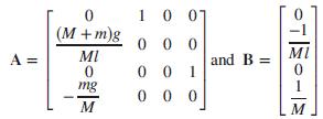
An inverted pendulum mounted on a motor-driven cart was presented in Problem 30 of Chapter 3. The nonlinear state-space equations representing that system were linearized (Prasad, 2012) around a stationary point corresponding to the pendulum point-mass, m, being in the upright position (x₀ = 0 at t = 0), when the force applied to the cart was zero (u₀ = 0). The state-space model developed in that problem is

ẋ = Ax + Bu

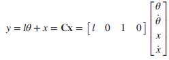
The state variables are the pendulum angle relative to the y-axis, θ, its angular speed, θ´, the horizontal position of the cart, x, and its speed, x´. The horizontal position of m(for a small angle, θ), x_m = x + l sin θ = x + lθ, was selected to be the output variable.

Given the state-space model developed in that problem along with the output equation you developed in that problem, use MATLAB (or any other computer program) to find and plot the output, x_m(t), in meters, for an input force, u(t), equal to a unit impulse, δ(t),in Newtons.

Data from Problem 30 of Chapter 3:

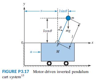
Figure P3.17 shows a free-body diagram of an inverted pendulum, mounted on a cart with a mass, M. The pendulum has a point mass, m, concentrated at the upper end of a rod with zero mass, a length, l, and a frictionless hinge. A motor drives the cart, applying a horizontal force, u(t). A gravity force, mg, acts on m at all times. The pendulum angle relative to the y-axis, θ, its angular speed, θ̇´, the horizontal position of the cart, x, and its speed, x´, were selected to be the state variables. The state-space equations derived were heavily nonlinear.¹⁴ They were then linearized around the stationary point, x₀ = 0 and u₀ = 0, and manipulated to yield the following open-loop model written in perturbation form: Figure P3.17 shows a free-body diagram of an inverted pendulum, mounted on a cart with a mass, M. The pendulum has a point mass, m, concentrated at the upper end of a rod with zero mass, a length, l, and a frictionless hinge. A motor drives the cart, applying a horizontal force, u(t). A gravity force, mg, acts on m at all times. The pendulum angle relative to the y-axis, θ, its angular speed, θ̇´ , the horizontal position of the cart, x, and its speed, x´, were selected to be the state variables. The state-space equations derived were heavily nonlinear.¹⁴ They were then linearized around the stationary point, x₀ = 0 and u₀ = 0, and manipulated to yield the following open loop model written in perturbation form:

However, since x₀ = 0 and u₀ = 0, then let: x = x₀ + δx = δx and u = u₀ + δ_u = δu. Thus the state equation may be rewritten as (Prasad, 2012):

ẋ = Ax + Bu

where

Assuming the output to be the horizontal position of m = x_m = x + l sinθ = x + lθ for a small angle, θ, the output equation becomes:

Given that: M = 2.4 kg, m = 0.23 kg, l = 0.36 m, g = 9.81 m/s², use MATLAB to find the transfer function, G(s)= Y(s)/U(s)= Xm(s)/U(s).

Transcribed Image Text:

d -Sx = Aôx + Bdu dt