Figure P8.15 shows a simplified drawing of a feedback system that includes the drive system presented in

Question:

Figure P8.15 shows a simplified drawing of a feedback system that includes the drive system

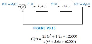
presented in Problem 67, Chapter 5 (Thomsen, 2011). Referring to Figures P5.43 and P8.15, Gp(s) in Figure P8.15 is given by:

Given that the controller is proportional, that is, G_C(s)= K_P, use MATLAB and a procedure similar to that developed in Problem 40 in this chapter to plot the root locus4 and obtain the output response, c(t) = ω_L(t), when a step input, r(t)= ω_r (t) = 260 u(t) rad/ sec, is applied at t = 0. Mark on the time response graph, c(t), all relevant characteristics, such as the percent overshoot (which should not exceed 16%), peak time, rise time, settling time, and final steady-state value.

Data From Problem 67, Chapter 5:

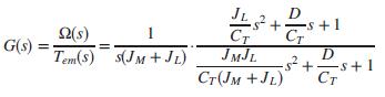
A drive system with an elastically coupled load was presented in Problem 71, Chapter 4. The mechanical part of this drive (Thomsen, 2011) was reduced to a two-inertia model. Using slightly different parameters, the following transfer function results:

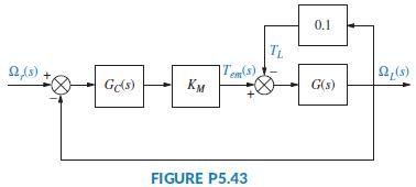
Here, T(s) = T_em(s) - T_L(s), where T_em (s) = the electromagnetic torque developed by the motor, T_L(s) = the load torque, and Ω_L(s) = the load speed. The drive is shown in Figure P5.43 as the controlled unit in a feedback control loop, where Ω_r(s) = the desired (reference) speed. The controller transfer function is G_C(s) = K_p + K_I/s = 4 + 0.5/s and provides an output voltage = 0 – 5.0 volts. The motor and its power amplifier have a gain, K_M = 10 N-m/volt.

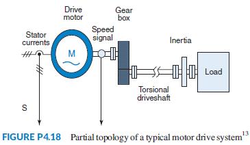
Data From Problem 71, Chapter 4:

A drive system with elastically coupled load (Figure P4.18) has a motor that is connected to the load via a gearbox and a long shaft. The system parameters are: J_M = drive-side inertia= 0.0338 kg-m², J_L = load-side inertia = 0.1287 kg-m², K = C_T = torsional spring constant = 1700 N-m/rad, and D = damping coefficient = 0.15 N-m-s/rad. This system can be reduced to a simple two inertia model that may be represented by the following transfer function, relating motor shaft speed output, Ω(s), to electromagnetic torque input (Thomsen, 2011):

Assume the system is at standstill at t = 0, when the electromagnetic torque, T_em, developed by the motor changes from zero to 50 N-m. Find and plot on one graph, using MATLAB or any other program, the motor shaft speed, ω(t), rad/sec, for the following two cases: