

We have already determined the expected returns and standard deviations for both Supertech and Slowpoke. In addition,
Question:
We have already determined the expected returns and standard deviations for both Supertech and Slowpoke. In addition, we calculated the deviation of each possible return from the expected return for each firm. Using this data, we can calculate covariance in two steps. An extra step is needed to calculate correlation.
1. For each state of the economy, multiply Supertech’s deviation from its expected return by Slowpoke’s deviation from its expected return. Supertech’s rate of return in a depression is −.20, which is − .375 ( = − .20 − .175 ) from its expected return. Slowpoke’s rate of return in a depression is .05, which is −.005 (= .05 − .055) from its expected return. Multiplying the two deviations together yields .001875 [= (−.375) × (−.005)]. The actual calculations are given in the last column of Table 11.2. This procedure can be written algebraically as:
Equation 11.2![]()
where R Super and RSlow are the returns on Supertech and Slowpoke in that state of the economy. E(RSuper) and E(RSlow) are the expected returns on the two securities.
2. Calculate the average value of the four states in the last column. This average is the covariance.
That is:![]()
Note that we represent the covariance between Supertech and Slowpoke as either Cov( R Super , RSlow) or σSuper, Slow. Equation 11.2 illustrates the intuition of covariance. Suppose Supertech’s return is generally above its average when Slowpoke’s return is above its average, and Supertech’s return is generally below its average when Slowpoke’s return is below its average.
This shows a positive dependency or a positive relationship between the two returns. Note that the term in Equation 11.2 will be positive in any state where both returns are above their averages. In addition, Equation 11.2 will still be positive in any state where both terms are below
Table 11.2 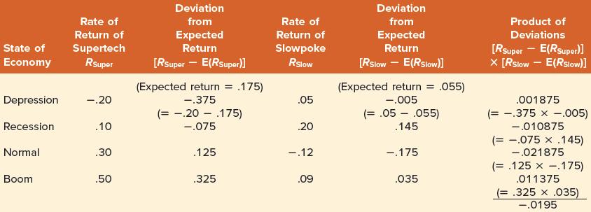
their averages. A positive relationship between the two returns will give rise to a positive value for covariance.
Conversely, suppose Supertech’s return is generally above its average when Slowpoke’s return is below its average, and Supertech’s return is generally below its average when Slowpoke’s return is above its average. This demonstrates a negative dependency or a negative relationship between the two returns. Note that the term in Equation 11.2 will be negative in any state where one return is above its average and the other return is below its average.
A negative relationship between the two returns will give rise to a negative value for covariance.
Finally, suppose there is no relationship between the two returns. In this case, knowing whether the return on Supertech is above or below its expected return tells us nothing about the return on Slowpoke. In the covariance formula, then, there will be no tendency for the deviations to be positive or negative together. On average, they will tend to offset each other and cancel out, making the covariance zero.
Of course, even if the two returns are unrelated to each other, the covariance formula will not equal zero exactly in any actual history. This is due to sampling error; randomness alone will make the calculation positive or negative. But for a historical sample that is long enough, if the two returns are not related to each other, we should expect the covariance to come close to zero.
The covariance formula seems to capture what we are looking for. If the two returns are positively related to each other, they will have a positive covariance, and if they are negatively related to each other, the covariance will be negative. Last, and very important, if they are unrelated, the covariance should be zero.
The formula for covariance can be written algebraically as:![]()
where E(R Super) and E(RSlow) are the expected returns on the two securities and RSuper and RSlow are the actual returns. The ordering of the two variables is unimportant. That is, the covariance of Supertech with Slowpoke is equal to the covariance of Slowpoke with Supertech. This can be stated more formally as Cov(RA,RB) = Cov(RB,RA) or σAB = σBA.
The covariance we calculated is −.004875. A negative number like this implies that the return on one stock is likely to be above its average when the return on the other stock is below its average, and vice versa. However, the size of the number is difficult to interpret. Like the variance figure, the covariance is in squared deviation units. Until we can put it in perspective, we don’t know what to make of it.
We solve the problem by computing the correlation.
3. To calculate the correlation, divide the covariance by the product of the standard deviations of both of the two securities. For our example, we have:
where σSuper and σSlow are the standard deviations of Supertech and Slowpoke, respectively. Note that we represent the correlation between Supertech and Slowpoke either as Corr(RSuper, RSlow) or ρSuper,Slow. As with covariance, the ordering of the two variables is unimportant. That is, the correlation of A with B is equal to the correlation of B with A. More formally, Corr (RA,RB) = Corr(RB,RA) or ρAB = ρBA. Because the standard deviation is always positive, the sign of the correlation between two variables must be the same as that of the covariance between the two variables. If the correlation is positive, we say that the variables are positively correlated; if it is negative, we say that they are negatively correlated; and if it is zero, we say that they are uncorrelated. Furthermore, it can be proven that the correlation is always between +1 and −1. This is due to the standardizing procedure of dividing by the product of the two standard deviations.
We also can compare the correlation between different pairs of securities. For example, it turns out that the correlation between General Motors and Ford is much higher than the correlation between General Motors and IBM. Hence, we can state that the first pair of securities is more interrelated than the second pair.
Figure 11.1 shows the three benchmark cases for two assets, A and B. The figure shows two assets with return correlations of +1, −1, and 0. This implies perfect positive correlation, perfect negative correlation, and no correlation, respectively. The graphs in the figure plot the separate returns on the two securities through time.
Figure 11.1 Examples of Different Correlation Coefficients: Graphs Plotting the Separate Returns on Two Securities through Time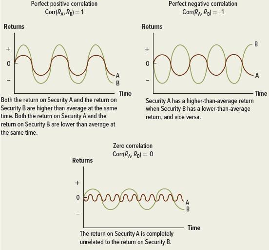
Step by Step Answer:
The provided text equations and images outline the process of calculating the covariance and correlation between two securities Supertech and Slowpoke ...View the full answer


Corporate Finance
ISBN: 9781265533199
13th International Edition
Authors: Stephen Ross, Randolph Westerfield, Jeffrey Jaffe
