Estimating the capital asset pricing model (CAPM). In Section 6.1 we considered briefly the well-known capital asset pricing model of modern portfolio theory. In empirical analysis, the CAPM is estimated in two stages.

Stage I (Time-series regression). For each of the N securities included in the sample, we run the following regression over time:

R_it = α̂_i + β̂_i R_mt + e_it €¦€¦€¦€¦€¦€¦. (1)

where R_it and R_mt are the rates of return on the ith security and on the market portfolio (say, the S&P 500) in year t; β_i , as noted elsewhere, is the Beta or market volatility coefficient of the ith security, and e_it are the residuals. In all there are N such regressions, one for each security, giving therefore N estimates of β_i.

Stage II (Cross-section regression). In this stage we run the following regression over the N securities:

RÌ…_i = γ̂₁ + γ̂₂ β̂_i + u_i €¦€¦€¦€¦€¦€¦.. (2)

where R̅_i is the average or mean rate of return for security i computed over the sample period covered by Stage I, β̂_i is the estimated beta coefficient from the first-stage regression, and u_i is the residual term.

Comparing the second-stage regression (2) with the CAPM Eq. (6.1.2), written as

ER_i = r_f + β_i(ER_m ˆ’ r_f ) €¦€¦€¦€¦.. (3)

where r_f is the risk-free rate of return, we see that γ̂₁ is an estimate of rf and γ̂₂ is an estimate of (ER_m ˆ’ r_f ), the market risk premium.

Thus, in the empirical testing of CAPM, RÌ…_i and β̂_i are used as estimators of ER_i and β_i, respectively. Now if CAPM holds, statistically,

γ̂₁ = r_f

γ̂₂ = R_m ˆ’ r_f, the estimator of (ER_m ˆ’ r_f)

Next consider an alternative model:

RÌ…_i = γ̂₁ + γ̂₂ Î²Ì‚_i + γ̂₃s²_ei + u_i €¦€¦€¦€¦€¦. (4)

where s²_ei is the residual variance of the ith security from the first-stage regression.

Then, if CAPM is valid, γˆ3 should not be significantly different from zero.

To test the CAPM, Levy ran regressions (2) and (4) on a sample of 101 stocks for the period 1948€“1968 and obtained the following results:

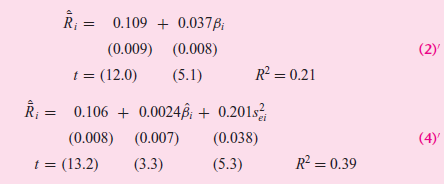
a. Are these results supportive of the CAPM?

b. Is it worth adding the variable s²_ei to the model? How do you know?

c. If the CAPM holds, γ̂₁ in (2)' should approximate the average value of the risk free rate, r_f. The estimated value is 10.9 percent. Does this seem a reasonable estimate of the risk-free rate of return during the observation period, 1948€“1968? (You may consider the rate of return on Treasury bills or a similar comparatively risk-free asset.)

d. If the CAPM holds, the market risk premium ( RÌ…_m ˆ’ r_f ) from (2)' is about 3.7 percent. If r_f is assumed to be 10.9 percent, this implies RÌ…_m for the sample period was about 14.6 percent. Does this sound like a reasonable estimate?

e. What can you say about the CAPM generally?

0.109 + 0.037i Ri %3D (0.009) (0.008) (2) R = 0.21 t = (12.0) (5.1) ; = 0.106 + 0.0024; + 0.201s, (4) (0.008) (0.007) (0.038) R = 0.39 (3.3) t = (13.2) (5.3) I|