Refer to the child mortality example discussed in Chapter 8 (Example 8.1). The example there involved the regression of the child mortality (CM) rate on per capita GNP (PGNP) and female literacy rate (FLR). Now suppose we add the variable, total fertility rate (TFR). This gives the following regression results.

a. Compare these regression results with those given in Eq. (8.1.4). What changes do you see? How do you account for them?
b. Is it worth adding the variable TFR to the model? Why?
c. Since all the individual t coefficients are statistically significant, can we say that we do not have a collinearity problem in the present case?

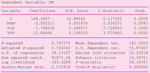
Dependent Variable: CM Variable Coefficient Std. Error t-Statistic Prob. 5.117003 0.0000 168.3067 32.89165 -2.934275 -0.005511 0.001878 0.0047 PGNP -1.768029 0.248017 -7.128663 0.0000 FLR 12.86864 4.190533 3.070883 0.0032 TFR Mean dependent var. S.D. dependent var. R-squared 0.747372 141.5000 Adjusted R-squared 0.734740 75.97807 S.E. of regression 39.13127 Akaike info criterion 10.23218 Sum squared resid. Log likelihood 91875.38 Schwarz criterion 10.36711 -323.4298 F-statistic 59.16767 2.170318 Durbin-Watson stat. Prob (F-statistic) 0.000000