

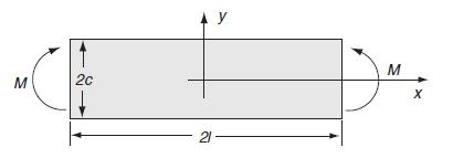
Question: 7.13 For the pure bending problem shown in Example 8.2 , the plane stress displacement field was determined and given by relations (8.1.22) 2 as:
7.13 For the pure bending problem shown in Example 8.2 , the plane stress displacement field was determined and given by relations (8.1.22)2 as:
![]()
Equation 8.1 .22
![0x = u = M Mxy EI dy = Txy = 0 M 2EI V= [vy + x-]](https://dsd5zvtm8ll6.cloudfront.net/images/question_images/1704/9/6/5/579659fb5cb6af7c1704965578187.jpg)
Using the appropriate transformation relations from Table7.1 , determine the corresponding displacements for the plane strain case. Next develop a comparison plot for each case of the y-displacement along the x-axis (y = 0) with Poisson’s ratio v = 0.4 . Use dimensionless variables and plot v(x, 0)/(Ml2/EI) versus x/l. Which displacement is larger and what happens as Poisson’s ratio goes to zero?
Table 7.1
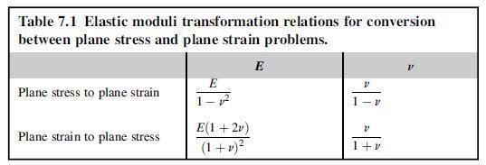
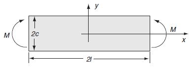
Data from example 8.2 As a second plane stress example, consider the case of a straight beam subjected to end moments as shown in Fig.8.2 . The exact pointwise loading on the ends only involve the specification of shear stress while end normal stress distribution is specified by the statically equivalent effect of zero force and moment. Hence, the boundary conditions on this problem are written as:
Fig 8.2
Thus, the boundary conditions on the ends of the beam have been relaxed, and only the statically equivalent condition for sx will be satisfied. This fact leads to a solution that is not necessarily valid near the ends of the beam.
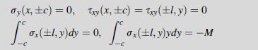
The choice of stress function is based on the fact that a third-order function will give rise to a linear stress field, and a particular linear boundary loading on the ends x =± l will reduce to a pure moment. Based on these two concepts, we choose:
This field automatically satisfies the boundary conditions on y =± c and gives zero net forces at the ends of the beam. The remaining moment conditions at x =± l are satisfied if A03 =–M/4c3, and thus the stress field is determined as:
![]()
The displacements are again calculated in the same fashion as in the previous example.
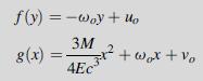
Assuming plane stress, Hooke’s law will give the strain field, which is then substituted into the strain-displacement relations and integrated, yielding the result:
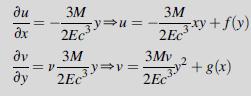
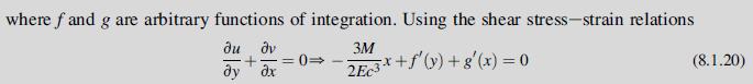
this result can again be separated into two independent relations in x and y, and upon integration the arbitrary functions f and g are determined as:
Again, rigid-body motion terms are brought out during the integration process. For this problem, the beam would normally be simply supported, and thus the fixity displacement boundary conditions could be specified as v(± l,0) = 0 and u(–l,0) = 0. This specification leads to determination of the rigid-body terms as uo = ωo = 0, vo =–3Ml2/4Ec3.
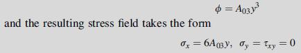
We now wish to compare this elasticity solution with that developed by elementary strength of materials (often called mechanics of materials). Appendix D, Section D.3, conveniently provides a brief review of this undergraduate theory. Introducing the cross-sectional area moment of inertia I = 2c3/3 (assuming unit thickness), our stress and displacement field can be written as:
![0x = U= M Mxy dy = Txy = 0 M [vy + x ] 2EI](https://dsd5zvtm8ll6.cloudfront.net/images/question_images/1704/9/6/5/443659fb54366ce91704965442224.jpg)
Note that for this simple moment-loading case, we have verified the classic assumption from elementary beam theory that plane sections remain plane. Note, however, that this will not be the case for more complicated loadings. The elementary strength of materials solution is obtained using Euler–Bernoulli beam theory and gives the bending stress and deflection of the beam centerline as:
![0x = M T v = v(x,0) = dy = Txy = 0 M 2E1 [x-]](https://dsd5zvtm8ll6.cloudfront.net/images/question_images/1704/9/6/5/493659fb575d7b261704965492531.jpg)
Comparing these two solutions, it is observed that they are identical, with the exception of the x displacements. In general, however, the two theories will not match for other beam problems with more complicated loadings, and we investigate such a problem in the next example.
U = Mxy V = M = [vy + x-1], -1x1 2EI
Step by Step Solution
3.47 Rating (150 Votes )
There are 3 Steps involved in it
Mxy Plane Stress Plane Strain E Plane Stress Results Al... View full answer

Get step-by-step solutions from verified subject matter experts