Let us consider an activity, whose level is measured by a continuous decision variable. A concrete example would be the amount of an asset that we purchase. The cost of the activity may include both a fixed charge f and a variable component

c. By a fixed charge, we mean a cost that is incurred whenever x > 0, in which case the cost does not depend on the specific level x of the activity. Note that this is not the same as a fixed (sunk) cost that is always paid for whatever level x, including x = 0. The cost function is

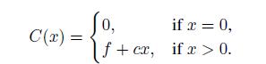
This function is discontinuous at the origin, and it is clearly not convex.
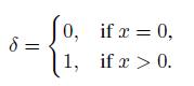
We may express the cost within an LP framework by introducing an auxiliary binary decision variable , related to x:

If we introduce a suitably large constant M, playing the role of an upper bound on x, we may relate the continuous variable x and the binary variable by a linear inequality:

If we introduce a suitably large constant M, playing the role of an upper bound on x, we may relate the continuous variable x and the binary variable by a linear inequality:

To see how this works, observe that if = 0, then x is forced down to zero, whereas the bound x M is enforced when = 1. This bound is irrelevant if M is large enough. Then, cost is expressed by the linear function

It may be argued that this does not forbid the nonsensical case in which we pay the fixed charge

f, but leave x = 0. However, it is easy to see that such a solution will never be optimal. This kind of modeling trick is called big-M constraint, as we require a suitably large M (when no sensible bound can be devised). From a computational viewpoint, the smaller the big-M, the better, as we shall see later.

0.