Let us consider two assets, \(a\) and \(b\), with current price

\[S_{a}(0)=S_{b}(0)=1\]

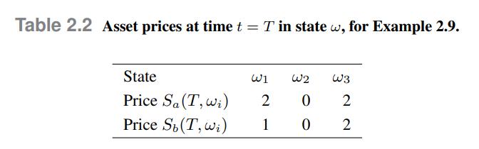
at time \(t=0\). At a later time \(t=T\), the asset prices, denoted by  and are random variables whose value depends on the realized scenario . Let us assume that there are three possible scenarios \(i, i=123\), with prices given in Table 2.2. Let us consider a portfolio in which we hold an amount \(h_{a}\) and \(h_{b}\) of the two assets, respectively. We notice that profit/loss is given as follows, depending on the scenario/state of nature:

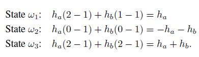
If we choose \(h_{a}=1\) and \(h_{b}=1\), the net cash flow at \(t=0\) is zero, we have a profit in state 1 , and no profit/loss is incurred in the remaining states. More generally, in this example any portfolio with \(h_{a}+h_{b}=0, h_{a}>0\), is an arbitrage strategy.

We may observe that the source of the anomaly is that asset \(a\) dominates asset \(b\), state by state. We will consider conditions precluding this anomaly.

Data From Table 2.2

Transcribed Image Text:

Sa(T,w)