Modify the Mathcad program in Figure 3.6 to repeat Example 3.9, but with $y_{A, G}=0.70$ and $x_{A,
Question:
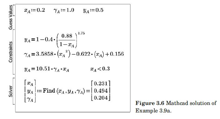
Modify the Mathcad program in Figure 3.6 to repeat Example 3.9, but with $y_{A, G}=0.70$ and $x_{A, L}=0.10$. Everything else remains constant.
Data From Example 3.9:-
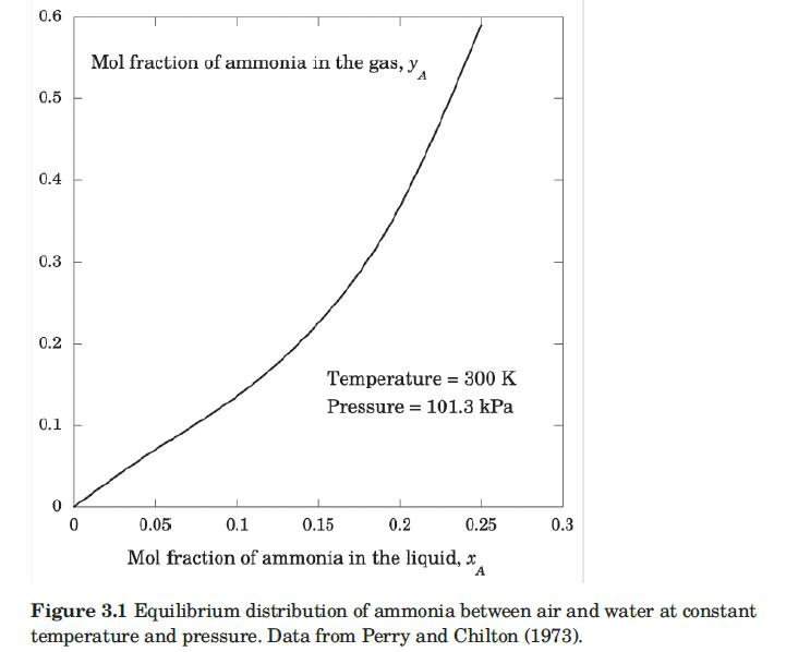
A wetted-wall absorption tower is fed with water as the wall liquid and an ammonia– air mixture as the central-core gas. At a particular point in the tower, the ammonia concentration in the bulk gas is 0.60 mol fraction, that in the bulk liquid is 0.12 mol fraction. The temperature is 300 K, and the pressure is 1 atm. Ignoring the vaporization of water, calculate the local ammonia mass-transfer flux. The rates of flow are such that FL = 3.5 mol/m2-s, and FG = 2.0 mol/m2-s. The equilibrium- distribution data for the system at 300 K and 1 atm are those shown graphically in Figure 3.1, and algebraically in Example 3.3.
Figure 3.6:-
Data From Example 3.3:-
Ten kilograms of dry gaseous ammonia, NH3, and 15 m3 of dry air measured at 300 K and 1 atm are mixed together and then brought into contact with 45 kg of water at 300 K in a piston/cylinder device. After a long period of time, the system reaches equilibrium. Assuming that the temperature and pressure remain constant, calculate the equilibrium concentrations of ammonia in the liquid and gas phases. Assume that the amount of water that evaporates and the amount of air that dissolves in the water are negligible. At 300 K and 1 atm, the equilibrium solubility of ammonia in air can be described with PA = 10.51 atm, and the activity coefficient of ammonia given by (for xA
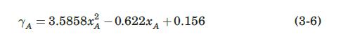
Figure 3.1:-
Step by Step Answer: