Reconsider the Truffle supply and demand model in Example 11.1. Suppose we modify the supply equation to be \(Q_{i}=\beta_{1}+\beta_{2} P_{i}+e_{i}^{s}\), keeping the demand equation unchanged.

a. Are the supply and demand equations identified using the necessary condition in Section 11.4? Explain.

b. The estimated first-stage, reduced form, equation becomes

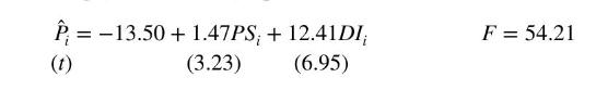
Do you judge the omitted exogenous variables (instruments) strong enough to estimate the identified equation(s)? Explain.

c. The estimated supply equation using 2 SLS is

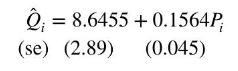
Verify that the point of the means (see Table 11.1) falls on the estimated supply curve.

d. Calculate the price elasticity of supply at the means and compare it to the elasticity computed from the 2SLS estimates in Table 11.3b.

e. Comparing the results in parts (b) and (c) to those in Example 11.1, do you think we should include \(P F\) in the supply equation? Explain.

Data From Example 11.1:-

Truffles are a gourmet delight. They are edible fungi that grow below the ground. In France they are often located by collectors who use pigs to sniff out the truffles and "point" to them. Actually the pigs dig frantically for the truffles because pigs have an insatiable taste for them, as do the French, and they must be restrained from "pigging out" on them. Consider a supply and demand model for truffles:

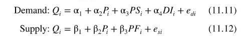
In the demand equation \(Q\) is the quantity of truffles traded in a particular French marketplace, indexed by \(i, P\) is the market price of truffles, \(P S\) is the market price of a substitute for real truffles (another fungus much less highly prized), and \(D I\) is per capita monthly disposable income of local residents. The supply equation contains the market price and quantity supplied. Also it includes \(P F\), the price of a factor of production, which in this case is the hourly rental price of truffle-pigs used in the search process. In this model, we assume that \(P\) and \(Q\) are endogenous variables. The exogenous variables are \(P S\), \(D I, P F\), and the intercept.

Before thinking about estimation, check the identification of each equation. The rule for identifying an equation is that in a system of \(M\) equations at least \(M-1\) variables must be omitted from each equation in order for it to be identified. In the demand equation the variable \(P F\) is not included; thus the necessary \(M-1=1\) variable is omitted. In the supply equation both \(P S\) and \(D I\) are absent; more than enough to satisfy the identification condition. Note too that the variables that are omitted are different for each equation, ensuring that each contains at least one shift variable not present in the other. We conclude that each equation in this system is identified and can thus be estimated by two-stage least squares.
Why are the variables omitted from their respective equations? Because economic theory says that the price of a factor of production should affect supply but not demand, and that the price of substitute goods and income should affect demand and not supply. The specifications we used are based on the microeconomic theory of supply and demand.

The reduced-form equations express each endogenous variable, \(P\) and \(Q\), in terms of the exogenous variables \(P S, D I\), \(P F\), and the intercept, plus an error term. They are

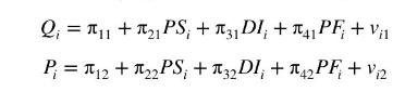
We can estimate these equations by OLS since the right-hand side variables are exogenous and contemporaneously uncorrelated with the random errors \(v_{i 1}\) and \(v_{i 2}\). The data file

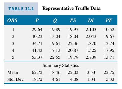
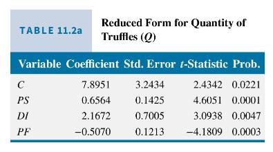
truffles contains 30 observations on each of the endogenous and exogenous variables. The units of measurement are \(\$\) per ounce for price \(P\), ounces for \(Q, \$\) per ounce for \(P S\), and thousands of dollars for \(D I ; P F\) is the hourly rental rate \((\$)\) for a truffle-finding pig. A few of the observations are shown in Table 11.1. The results of the least squares estimations of the reduced-form equations for \(Q\) and \(P\) are reported in Tables \(11.2 \mathrm{a}\) and \(11.2 \mathrm{~b}\).
In Table 11.2a, we see that the estimated coefficients are statistically significant, and thus we conclude that the exogenous variables affect the quantity of truffles traded, \(Q\), in this reduced-form equation. The \(R^{2}=0.697\), and the overall \(F\)-statistic is 19.973 , which has a \(p\)-value of less than 0.0001 . In Table \(11.2 \mathrm{~b}\) the estimated coefficients

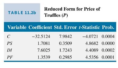
are statistically significant, indicating that the exogenous variables have an effect on market price \(P\). The \(R^{2}=0.889\) implies a good fit of the reduced-form equation to the data. The overall \(F\)-statistic value is 69.189 that has a \(p\)-value of less than 0.0001 , indicating that the model has statistically significant explanatory power.
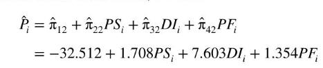
The reduced-form equations are used to obtain \(\hat{P}\) that will be used in place of \(P\) on the right-hand side of the supply and demand equations in the second stage of two-stage least squares. From Table 11.2b, we have

The 2SLS results are given in Tables 11.3a and 11.3b. The estimated demand curve results are in Table 11.3a. Note that the coefficient of price is negative, indicating that as the market price rises, the quantity demanded of truffles declines, as predicted by the law of demand. The standard errors that are reported are obtained from 2SLS software. They and the \(t\)-values are valid in large samples. The \(p\)-value indicates that the estimated slope of the demand curve is significantly different from zero. Increases in the price of the substitute for truffles increase the demand for truffles, which is a characteristic of substitute goods. Finally the effect of income is positive, indicating that truffles are a normal good. All of

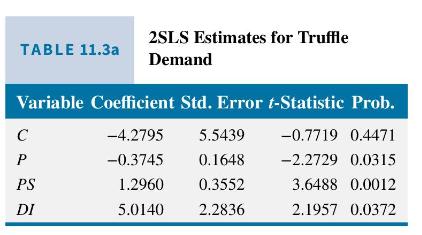
these variables have statistically significant coefficients and thus have an effect upon the quantity demanded.
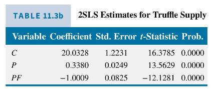
The supply equation results appear in Table 11.3b. As anticipated, increases in the price of truffles increase the quantity supplied, and increases in the rental rate for truffle-seeking pigs, which is an increase in the cost of a factor of production, reduces supply. Both of these variables have statistically significant coefficient estimates.

Transcribed Image Text:

(t) =-13.50+ 1.47PS; + 12.41DI; (3.23) (6.95) F = 54.21