Using the NLS panel data on \(N=716\) young women, we consider only years 1987 and 1988 . We are interested in the relationship between \(\ln (W A G E)\) and experience, its square, and indicator variables for living in the south and union membership. We form first differences of the variables, such as \(\Delta \ln (W A G E)=\ln \left(W A G E_{i, 1988}\right)-\ln \left(W A G E_{i, 1987}\right)\), and specify the regression

Table 15.11 reports OLS estimates of equation (XR15.7) as Model (1), with conventional standard errors in parentheses.

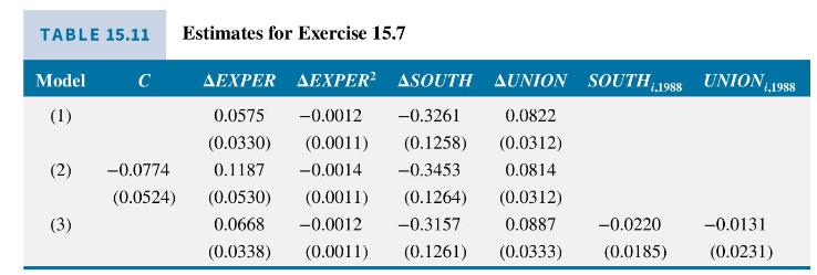
a. The ability of first differencing to eliminate unobservable time-invariant heterogeneity is illustrated in equation (15.8). Explain why the strict form of exogeneity, FE2, is required for the difference estimator to be consistent. You may wish to reread the start of Section 15.1.2 to help clarify the assumption.

b. Equation (XR15.6) is the panel data regression specification at the base of the difference model. Suppose we define the indicator variable \(D 88_{t}=1\) if the year is 1988 and \(D 88_{t}=0\) otherwise, and add it to the specification in equation (XR15.6). What would its coefficient measure?

c. Model (2) in Table 15.11 is the difference model including an intercept term. Algebraically show that the constant term added to the difference model is the coefficient of the indicator variable discussed in part (b). Is the estimated coefficient statistically significant at the 5\% level? What does this imply about the intercept parameter in equation (XR15.6) in 1987 versus 1988?

d. In the difference model, the assumption of strict exogeneity can be checked. Model (3) in Table 15.11 adds the variables SOUTH and UNION for year 1988 to the difference equation. As noted in equation (15.5a), the strict exogeneity assumption fails if the random error is correlated with the explanatory variables in any time period. We can check for such a correlation by including some, or all, of the explanatory variables for year \(t\), or \(t-1\) into the difference equation. If strict exogeneity holds these additional variables should not be significant. Based on the Model (3) result is there any evidence that the strict exogeneity assumption does not hold?

e. The F-test value for the joint significance of SOUTH and UNION from part (d), in Model (3), is 0.81 . Are the variables jointly significant? What are the test degrees of freedom? What is the \(5 \%\) critical value?

Data From Equation (XR15.6):-

Transcribed Image Text:

Aln(WAGE) BAEXPER+BAEXPER + BASOUTH+BAUNION + Ae (XR15.7) =