Some methods in this chapter are easy with technology but very difficult without it. The two projects that follow illustrate how easy it is to use technology for assessing normality and finding binomial probabilities.

1. Assessing Normality It is often necessary to determine whether sample data appear to be from a normally distributed population, and that determination is helped with the construction of a histogram and normal quantile plot. Refer to Data Set 1 “Body Data” in Appendix B. For each of the 13 columns of data (not including age or gender), determine whether the data appear to be from a normally distributed population. Use Statdisk or any other technology. (Download a free copy of Statdisk from www.statdisk.org.)
2. Binomial Probabilities Section 6-6 described a method for using a normal distribution to approximate a binomial distribution. Many technologies are capable of generating probabilities for a binomial distribution. Instructions for these different technologies are found in the Tech Center at the end of Section 5-2 on page 208. Instead of using a normal approximation to a binomial distribution, use technology to find the exact binomial probabilities in Exercises 9–12 of Section 6-6.

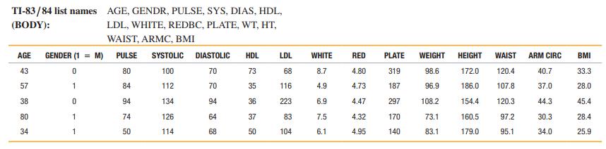
Data Set 1: Body Data

Body and exam measurements are from 300 subjects (first five rows shown here). AGE is in years, for GENDER 1 = male and 0 = female, PULSE is pulse rate (beats per minute), SYSTOLIC is systolic blood pressure (mm Hg), DIASTOLIC is diastolic blood pressure (mm Hg), HDL is HDL cholesterol (mg/dL), LDL is LDL cholesterol (mg/dL), WHITE is white blood cell count (1000 cells//mL), RED is red blood cell count (million cells/mL), PLATE is platelet count (1000 cells/mL), WEIGHT is weight (kg), HEIGHT is height (cm), WAIST is waist circumference (cm), ARM CIRC is arm circumference (cm), and BMI is body mass index (kg/m2). Data are from the National Center for Health Statistics.

In Exercises 9–12, assume that 100 cars are randomly selected. Refer to the accompanying graph, which shows the top car colors and the percentages of cars with those colors.

Data From Exercise 9 Section 6-6:

Find the probability that fewer than 20 cars are white. Is 20 a significantly low number of white cars?

Data From Exercise 10 Section 6-6:

Find the probability that at least 25 cars are black. Is 25 a significantly high number of black cars?

Data From Exercise 11 Section 6-6:

Find the probability of exactly 14 red cars. Why can’t the result be used to determine whether 14 is a significantly high number of red cars?

Data From Exercise 12 Section 6-6:

Find the probability of exactly 10 gray cars. Why can’t the result be used to determine whether 10 is a significantly low number of gray cars?