Compute and plot the Jacobian \(J(\eta ; t)\) and the \(\operatorname{Pdf} f(\varphi ; t)\) for \(t>0\) using the mapping \(\mathcal{X}(\eta ; t)\) of the previous problem 13.1.

Problem 13.1

Compute the analytic solution of the IVP for the mapping pde (13.23) for a single conserved \((Q(\eta)=0)\) scalar. The scalar space is the unit interval \(\mathcal{R}_{\Phi}=\) \([0,1]\), and the initial condition is

\[ \mathcal{X}(\eta ; 0)=\sum_{k=1}^{N} w_{k} H\left(\eta-\eta_{k}\right), w_{k} \geq 0, \sum_{k=1}^{N} w_{k}=1 \]

where \(H\left(\eta-\eta_{k}\right)\) denotes the unit step function located at \(\eta_{k}\).

13.1.1: Rescale the time variable \(t\) to transform the mapping pde to the form

\[ \left(\frac{\partial}{\partial \tau}+\eta \frac{\partial}{\partial \eta}-\frac{\partial^{2}}{\partial \eta^{2}}\right) \mathcal{X}(\eta, \tau)=0 \]

13.1.2: Transform the scalar variable using \(\tilde{\eta} \equiv \eta \exp (-\tau)\) to obtain a new pde for \(\mathcal{X}\).

13.1.3: Solve the new pde for \(\mathcal{X}\). The Green's function approach is recommended, see Duffy [9], Sect. 4.1 for details.

13.1.4: Plot the solution \(\mathcal{X}(\eta ; t)\) for several times in [0, 0.3].

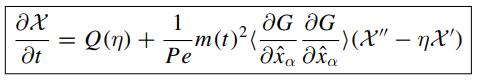
pde (13.23)

Transcribed Image Text:

ax 1 AG OG = Q(n) + -m(t) ( - It Pe