1) In cell E4, create a formula that calculate the Profit Margin % and copy that formula down to E28. Format the values to show the percent value with zero decimal places (i.e.24%) 2) In cell F4, create a formula that calculates the Total Cost and copy that formula down to F28. Remember from above to apply the Currency format to all of the lines with zero decimal places but only show the $ sign on the top row! 3) In cell G4, create a formula that calculates the Total Sales to Dealer using the logic above and copy that formula down to G28 4) For % of Total Volume in column H, first calculate the total volume of all cars sold in cell B30. Then in cell H4, for that model, find the % of its volume as compared to the Total Volume now located in B30. For full credit, you should write your formula in H4 using proper cell referencing (hint: Mixed referencing puts the $ sign in front of either the column OR the row and absolute referencing puts $ signs in front of both column AND row. One of these two techniques is the better/more efficient choice so that is the one that will get you the most points! By using proper as you copy/paste the formula down for all models, Excel properly writes the formula in all of the cells.

Format the cells in column H to display percentage values to the nearest tenth of a percent (e.g. 5.6%).

5) In row 30, calculate the totals for each of the 3 shaded columns (B, F & G) 6) For row 31, Calculate the averages for all columns except for the Profit Margin (since that would require a weighted average and that is for a later module). Mentally make a note of what the AVERAGE formula calculates for the columns with no number in them for sales. Now put zeroes into the Sales Volume cells that are empty (NULL) and note the difference. Zero counts differently than empty/NULL! Leave in the zeroes for the rest of this Assignment because it is important to note that they did not sell any of those models! Display all average values (other than the percentage) with commas and no decimal places and $ signs if appropriate.

7) In cells B32 and B33 write a formula that finds the highest and lowest volumes of all of the car models. Format these with commas and no decimal places. 8) In cell E35 write a formula that provides the number of different models that are available regardless of whether there were sales for that model or not (hint: you will need to use the "Model" column in order to do this because that is the only column that will always contain data for each model). You will need to use the formula that counts cells containing text (i.e. MO307).

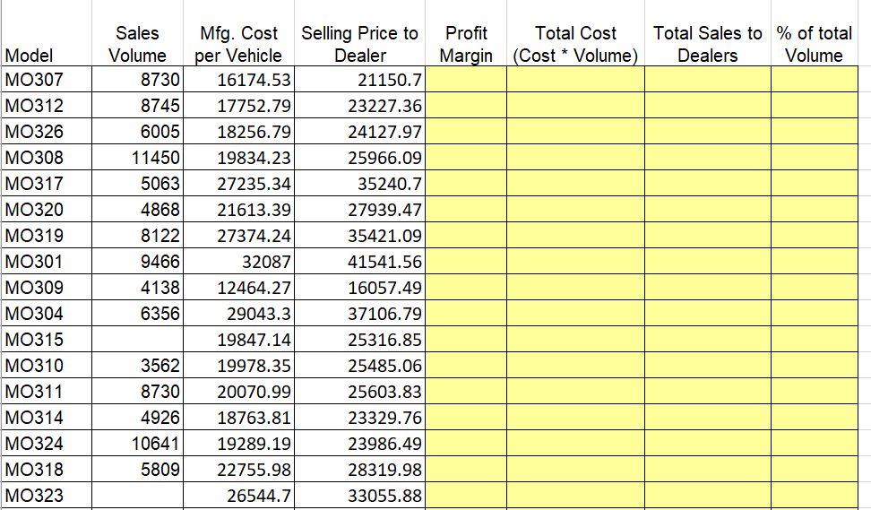
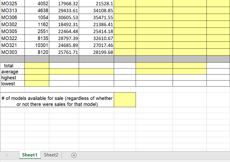
Sales Mfg. Cost Selling Price to Profit Total Cost Total Sales to % of total Margin (Cost Volume) Volume Model MO307 MO312 MO326 MO308 MO317 MO320 MO319 MO301 MO309 MO304 MO315 MO310 MO311 MO314 MO324 MO318 MO323 Dealer Dealers Volume per Vehicle 873016174.53 874517752.79 600518256.79 1145019834.23 506327235.34 486821613.39 812227374.24 32087 413812464.27 29043.3 19847.14 356219978.35 873020070.99 4926 18763.81 10641 19289.19 580922755.98 26544.7 21150.7 23227.36 24127.917 25966.09 35240.7 27939.47 35421.09 41541.56 16057.49 37106.79 25316.85 25485.06 25603.83 23329.76 23986.49 28319.98 33055.88 9466 6356