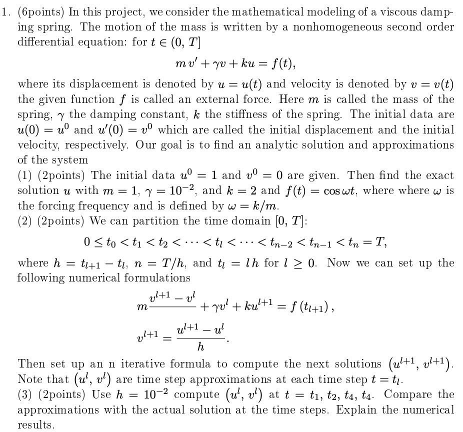
1. (points) In this project, we consider the mathematical modeling of a viscous damp- ing spring. The motion of the mass is written by a nonhomogeneous second order differential equation: for t E (0, T] mu' + y + ku = f(t), where its displacement is denoted by u = u(t) and velocity is denoted by v = v(t) the given function f is called an external force. Here m is called the mass of the spring, y the damping constant, k the stiffness of the spring. The initial data are u(0) = u' and u'(0) = v which are called the initial displacement and the initial velocity, respectively. Our goal is to find an analytic solution and approximations of the system (1) (2points) The initial data u = 1 and v = 0 are given. Then find the exact solution u with m = 1, y = 10-2, and k = 2 and f(t) = cos wt, where where w is the forcing frequency and is defined by w = k/m. (2) (2points) We can partition the time domain (0, T]: 0 0. Now we can set up the following numerical formulations me 22+1 01 =" + you? + ku?+1 = f (t1+1), v1+1 _ u'+1 - 21 Then set up an n iterative formula to compute the next solutions (u+1, 21+1). Note that (u, v) are time step approximations at each time step t=ti. (3) (2points) Use h = 10-2 compute (u', v') at t = ti, t2, t4, 14. Compare the approximations with the actual solution at the time steps. Explain the numerical results. 1. (points) In this project, we consider the mathematical modeling of a viscous damp- ing spring. The motion of the mass is written by a nonhomogeneous second order differential equation: for t E (0, T] mu' + y + ku = f(t), where its displacement is denoted by u = u(t) and velocity is denoted by v = v(t) the given function f is called an external force. Here m is called the mass of the spring, y the damping constant, k the stiffness of the spring. The initial data are u(0) = u' and u'(0) = v which are called the initial displacement and the initial velocity, respectively. Our goal is to find an analytic solution and approximations of the system (1) (2points) The initial data u = 1 and v = 0 are given. Then find the exact solution u with m = 1, y = 10-2, and k = 2 and f(t) = cos wt, where where w is the forcing frequency and is defined by w = k/m. (2) (2points) We can partition the time domain (0, T]: 0 0. Now we can set up the following numerical formulations me 22+1 01 =" + you? + ku?+1 = f (t1+1), v1+1 _ u'+1 - 21 Then set up an n iterative formula to compute the next solutions (u+1, 21+1). Note that (u, v) are time step approximations at each time step t=ti. (3) (2points) Use h = 10-2 compute (u', v') at t = ti, t2, t4, 14. Compare the approximations with the actual solution at the time steps. Explain the numerical results