Question: 18. (5 points) Compare model (5) with model (6), which is likely to have larger coefficient for male ? Explain why. 19. (5 points) Suppose

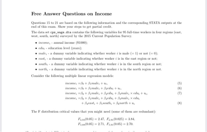
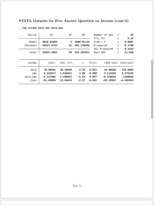
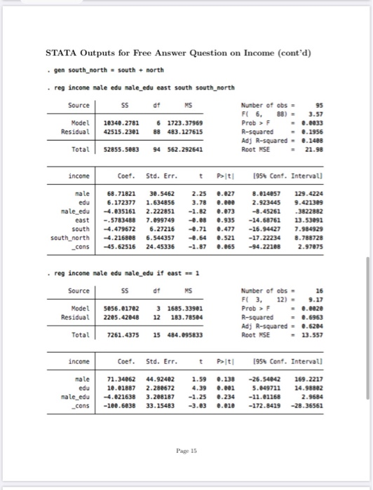
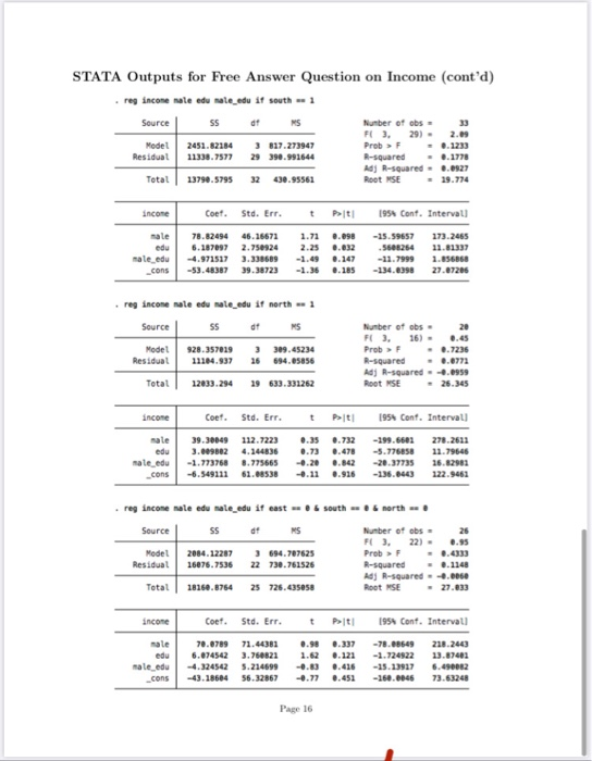
18. (5 points) Compare model (5) with model (6), which is likely to have larger coefficient for male ? Explain why. 19. (5 points) Suppose the R for model (6) is 0.1368. Which of the two models, (6) and (7), explains workers' annual income better? Why? Free Answer Questions on Income Questions 15 to 21 are based on the following information and the corresponding STATA outputs at the end of this exam. Show your steps to get partial credit The dataset cpa_wage.dta contains the following variables for 95 full-time workers in four regions (cast, west, south, north) surveyed by the 2015 Current Population Survey. income-annual income ($1000): edus - education level (years); male - a dummy variable indicating whether worker i in male (= 1) or not (=0); cast, - a dummy variable indicating whether worker i is in the east region or not; south-a dummy variable indicating whether worker is in the south region or not; worth - a dummy variable indicating whether worker i is in the north region or not. Consider the following multiple linear regression models: income, =+ Bimale+ income = 80+ Bimales + Bzedu. + (6) income, =B0+ male + Baedu,+Bymale, edu, + (7) income, =B6 + 8 male, + Byedu,+Bymale, X edu + Secasti + Ss south + Benorth + (8) The F distribution critical values that you might need some of them are redundant): F4.98(0.05) = 2.47. F. (0.025) = 3.84, F3.84(0.05) = 2.71, F.:(0.05) = 2.70. STATA Outputs for Free Answer Question on Labor Supply use labor_supply.dta gen thours .log(hours) reg thours wage Source ss MS Number of obs 428 F(1, 426) Model 7.74052955 1 7.74052955 Prob>F 0.0040 Residual 393.136648 426 .922855981 R-squared 0.0193 Adj R-squared 0.0170 Total 400.877178 427 .93882243 Root MSE .96065 thours Coef. Std. Err. t Pti 1954 Cont. Intervall wage cons -.040673 7.036879 .0140439 6748231 -.068277 6.889811 3069 7.183947 94.05 0.000 gen wage_non - wage . non reg thours non wage wage_non Source SS df NS Model Residual 13.9331379 386.94464 3 4.64437929 424.912683867 Number of obs F(3, 424) Prob > F R-squared Adj R-squared Root MSE 428 5.09 0.0018 0.0348 0.0279 9553 Total 400.877178 427 .93882243 Thours Coef. Std. Err. t Pt1 1954 Cont. Intervall no wage Wage_non cons -.0462971 -.0155766 -.0404024 7.075578 .1612755 0240036 . 0295331 .1341665 -0.29 -0.65 -1.37 52.74 0.774 0.517 0.172 -.3632963 -.0627575 -.0984519 6.811864 .270702 0316843 .0176472 7.339292 STATA Outputs for Free Answer Question on Income use cps_wage.de tab male, sun(income) nean Summary of annual income ($1828) Mean male dunny 40.1244 45.557636 1 Total 43.269958 . ttest income, bynale) Two-sample t test with equal variances Group Obs Mean Std. Err. Std. Dev. 1951 Cont. Intervall e 1 40.1244 45.55754 4.678401 2.972461 25.79407 22.03694 31.87506 39.68022 48.37374 51.51506 55 combined 95 43.26996 2.432873 23.71271 38.43943 48.10048 -5.433236 4.922837 -15.20703 4.340557 ditt mean(e) - mean(1) Ho: ditt = t. -1.1039 degrees of freedom Ha: ditt to PriT It|) = 0.2725 gennale_edule.edu Ha: ditt > Prit) - 0.8638 . reg edu male Source 55 df WS Model Residual 95.1751196 425.799891 1 95.1751195 93 4.36246334 Number of obs 95 FL 1. 93) 21.82 Prob = 0.0000 R-squared = 0.1900 Adj R-squared - 0.1813 Root MSE - 2.6887 Total see.884211 94 5.32855543 edu Coet. Std. Err. t ti 1954 Cont. Intervall -2.689164 -1.265382 13.8442 15.1558 sale -2.627273 14.5 cons .3382447 43.91.000 Page 13 STATA Outputs for Free Answer Question on Income (cont'd) . reg income nale edu nale_edu Source SS df MS Model Residual 9018.03405 43837.4742 3 3006.01135 91 481.730486 Number of obs F(3, 91) Prob F R-squared Ad) R-squared Root MSE 95 6.24 0.0007 0.1706 0.1433 21.948 Total 52855.5083 94 562.292641 income Coef. Std. Err. t P> 1958 Conf. Intervall male edu male.edu cons 70.90301 6.343517 -4.217982 -51.85659 30.20439 1.626921 2. 190947 23.84424 2.35 3.90 -1.93 -2.17 0.021 0.000 ..057 0.032 10.90569 3. 111839 -8.570029 -99.22025 130.9083 9.575195 . 1348658 -4.492933 Page 14 STATA Outputs for Free Answer Question on Income (conta) gen south_north-south h + north . reg income male edu male_edu east south south_north Source SS df MS Number of obs = 95 FI 6, 88) = 3.57 Model 10340.2781 6 1723.37969 Prob > F - 0.0833 Residual 42515.2301 88 483.127615 R-squared - 0.1956 Adj R-squared - 0.1408 Total 52855.5283 94 562.292641 Root MSE 21.98 income Coef. Std. Err. t P>t 1954 Cont. Intervall male edu male_edu cast south south_north 68.71821 6.172377 -4.035161 -.5783488 -4.479672 -4.216808 -45.62516 30.5462 1.634856 2.222851 7.099749 6.27216 6.544357 24.45336 2.25 3.78 -1.82 -0.08 -0.71 0.027 0.000 0.073 0.935 0.477 0.521 @.865 8.014857 2.923445 -8.45262 -14.68761 -16.94427 -17.22234 -94.22188 129.4224 9.421389 .3822882 13.53091 7.984929 8.788728 2.97075 cons -1.87 reg income male edu male_edu it east = 1 Source SS df NS Model 5856.61782 3 1685.33901 Residual 2205.42848 183.78504 Number of obs 16 FL 3, 12) 9.17 Prob > F -0.0020 R-squared = 2.6963 Adj R-squared - 0.6204 Root MSE 13.557 12 Total 7261.4375 15 484.095833 incone Coef. Std. Err. t P>It male edu male edu cons 71.34062 10.01887 -4.621638 -100.6838 44.92402 2.288672 3.208187 33. 15483 1.59 4.39 -1.25 -3.63 0.138 0.001 0.234 0.010 1954 Conf. Intervall -26.54042 169.2217 5.249711 14.98802 -11.01168 2.9684 -172.8419 -28.36561 Page 15 STATA Outputs for Free Answer Question on Income (cont'd) reg income nele edu male_edu if south - 1 Source SS df MS Number of obs FL 3, 29) - 2.09 Model 2451.82184 3 817.273947 Prob - 0.1233 Residual 11338.7577 29 390.991644 R-squared -0.1778 Adj R-squared. 0.0927 Total 13790.5795 430.95561 Root MSE 29.774 32 income Coet. Std. Err. t Pti 1954 Cont. Intervall 2.25 0.098 0.032 173.2465 11.61337 edu male.edu cons 78.82494 6.187097 -4.971517 -53.48387 46.16671 2.750924 3.338689 39.38723 -15.59657 .5608254 -11.7999 -134.6398 -1.36 0.185 27.67205 reg incone nale edu nale_edu if north - 1 Source SS Modet Residual 928.357019 11104.937 MS 3 309.45234 25 694.65856 Number of obs 20 FL 3, 16) Prob F 6.7236 R-squared ...0771 Adj R-squared --.1999 Root MSE 25.345 Total 12033.294 19 633.331262 incone Coet. Std. Err. t P> 1959 Cont. Intervall 0.35 ..732 ..478 278.2611 11.79646 male edu nale.edu cons 39.30049 3.609802 -1.773768 -6.549111 112.7223 4.244836 8.775665 61.68530 -199.6603 -5.776858 -20.37735 -136.6443 -0.11 ..916 122.9461 reg incone male edu male_edu if east-south-north Source SS dt MS Number of obs- FL 3. 22) - 6.95 Model 2084.12287 3 694.707625 Prob Residual 16076.7536 22 730.761528 R-squared -0.1148 Adj R-squared-6.00 Total 18160.8754 25 726.435058 Root MSE - 27.033 Incone Coet. Std. Err. t 70.6789 6.674542 nale edu nale_edu cons 71.44381 3.760821 5.214699 56.32867 6.337 .. 121 1954 Conf. Intervall -78.68549 223.2443 13.67401 -15.1.1917 6.490082 -160.0046 73.63248 -43.18684 ..451 Page 16 18. (5 points) Compare model (5) with model (6), which is likely to have larger coefficient for male ? Explain why. 19. (5 points) Suppose the R for model (6) is 0.1368. Which of the two models, (6) and (7), explains workers' annual income better? Why? Free Answer Questions on Income Questions 15 to 21 are based on the following information and the corresponding STATA outputs at the end of this exam. Show your steps to get partial credit The dataset cpa_wage.dta contains the following variables for 95 full-time workers in four regions (cast, west, south, north) surveyed by the 2015 Current Population Survey. income-annual income ($1000): edus - education level (years); male - a dummy variable indicating whether worker i in male (= 1) or not (=0); cast, - a dummy variable indicating whether worker i is in the east region or not; south-a dummy variable indicating whether worker is in the south region or not; worth - a dummy variable indicating whether worker i is in the north region or not. Consider the following multiple linear regression models: income, =+ Bimale+ income = 80+ Bimales + Bzedu. + (6) income, =B0+ male + Baedu,+Bymale, edu, + (7) income, =B6 + 8 male, + Byedu,+Bymale, X edu + Secasti + Ss south + Benorth + (8) The F distribution critical values that you might need some of them are redundant): F4.98(0.05) = 2.47. F. (0.025) = 3.84, F3.84(0.05) = 2.71, F.:(0.05) = 2.70. STATA Outputs for Free Answer Question on Labor Supply use labor_supply.dta gen thours .log(hours) reg thours wage Source ss MS Number of obs 428 F(1, 426) Model 7.74052955 1 7.74052955 Prob>F 0.0040 Residual 393.136648 426 .922855981 R-squared 0.0193 Adj R-squared 0.0170 Total 400.877178 427 .93882243 Root MSE .96065 thours Coef. Std. Err. t Pti 1954 Cont. Intervall wage cons -.040673 7.036879 .0140439 6748231 -.068277 6.889811 3069 7.183947 94.05 0.000 gen wage_non - wage . non reg thours non wage wage_non Source SS df NS Model Residual 13.9331379 386.94464 3 4.64437929 424.912683867 Number of obs F(3, 424) Prob > F R-squared Adj R-squared Root MSE 428 5.09 0.0018 0.0348 0.0279 9553 Total 400.877178 427 .93882243 Thours Coef. Std. Err. t Pt1 1954 Cont. Intervall no wage Wage_non cons -.0462971 -.0155766 -.0404024 7.075578 .1612755 0240036 . 0295331 .1341665 -0.29 -0.65 -1.37 52.74 0.774 0.517 0.172 -.3632963 -.0627575 -.0984519 6.811864 .270702 0316843 .0176472 7.339292 STATA Outputs for Free Answer Question on Income use cps_wage.de tab male, sun(income) nean Summary of annual income ($1828) Mean male dunny 40.1244 45.557636 1 Total 43.269958 . ttest income, bynale) Two-sample t test with equal variances Group Obs Mean Std. Err. Std. Dev. 1951 Cont. Intervall e 1 40.1244 45.55754 4.678401 2.972461 25.79407 22.03694 31.87506 39.68022 48.37374 51.51506 55 combined 95 43.26996 2.432873 23.71271 38.43943 48.10048 -5.433236 4.922837 -15.20703 4.340557 ditt mean(e) - mean(1) Ho: ditt = t. -1.1039 degrees of freedom Ha: ditt to PriT It|) = 0.2725 gennale_edule.edu Ha: ditt > Prit) - 0.8638 . reg edu male Source 55 df WS Model Residual 95.1751196 425.799891 1 95.1751195 93 4.36246334 Number of obs 95 FL 1. 93) 21.82 Prob = 0.0000 R-squared = 0.1900 Adj R-squared - 0.1813 Root MSE - 2.6887 Total see.884211 94 5.32855543 edu Coet. Std. Err. t ti 1954 Cont. Intervall -2.689164 -1.265382 13.8442 15.1558 sale -2.627273 14.5 cons .3382447 43.91.000 Page 13 STATA Outputs for Free Answer Question on Income (cont'd) . reg income nale edu nale_edu Source SS df MS Model Residual 9018.03405 43837.4742 3 3006.01135 91 481.730486 Number of obs F(3, 91) Prob F R-squared Ad) R-squared Root MSE 95 6.24 0.0007 0.1706 0.1433 21.948 Total 52855.5083 94 562.292641 income Coef. Std. Err. t P> 1958 Conf. Intervall male edu male.edu cons 70.90301 6.343517 -4.217982 -51.85659 30.20439 1.626921 2. 190947 23.84424 2.35 3.90 -1.93 -2.17 0.021 0.000 ..057 0.032 10.90569 3. 111839 -8.570029 -99.22025 130.9083 9.575195 . 1348658 -4.492933 Page 14 STATA Outputs for Free Answer Question on Income (conta) gen south_north-south h + north . reg income male edu male_edu east south south_north Source SS df MS Number of obs = 95 FI 6, 88) = 3.57 Model 10340.2781 6 1723.37969 Prob > F - 0.0833 Residual 42515.2301 88 483.127615 R-squared - 0.1956 Adj R-squared - 0.1408 Total 52855.5283 94 562.292641 Root MSE 21.98 income Coef. Std. Err. t P>t 1954 Cont. Intervall male edu male_edu cast south south_north 68.71821 6.172377 -4.035161 -.5783488 -4.479672 -4.216808 -45.62516 30.5462 1.634856 2.222851 7.099749 6.27216 6.544357 24.45336 2.25 3.78 -1.82 -0.08 -0.71 0.027 0.000 0.073 0.935 0.477 0.521 @.865 8.014857 2.923445 -8.45262 -14.68761 -16.94427 -17.22234 -94.22188 129.4224 9.421389 .3822882 13.53091 7.984929 8.788728 2.97075 cons -1.87 reg income male edu male_edu it east = 1 Source SS df NS Model 5856.61782 3 1685.33901 Residual 2205.42848 183.78504 Number of obs 16 FL 3, 12) 9.17 Prob > F -0.0020 R-squared = 2.6963 Adj R-squared - 0.6204 Root MSE 13.557 12 Total 7261.4375 15 484.095833 incone Coef. Std. Err. t P>It male edu male edu cons 71.34062 10.01887 -4.621638 -100.6838 44.92402 2.288672 3.208187 33. 15483 1.59 4.39 -1.25 -3.63 0.138 0.001 0.234 0.010 1954 Conf. Intervall -26.54042 169.2217 5.249711 14.98802 -11.01168 2.9684 -172.8419 -28.36561 Page 15 STATA Outputs for Free Answer Question on Income (cont'd) reg income nele edu male_edu if south - 1 Source SS df MS Number of obs FL 3, 29) - 2.09 Model 2451.82184 3 817.273947 Prob - 0.1233 Residual 11338.7577 29 390.991644 R-squared -0.1778 Adj R-squared. 0.0927 Total 13790.5795 430.95561 Root MSE 29.774 32 income Coet. Std. Err. t Pti 1954 Cont. Intervall 2.25 0.098 0.032 173.2465 11.61337 edu male.edu cons 78.82494 6.187097 -4.971517 -53.48387 46.16671 2.750924 3.338689 39.38723 -15.59657 .5608254 -11.7999 -134.6398 -1.36 0.185 27.67205 reg incone nale edu nale_edu if north - 1 Source SS Modet Residual 928.357019 11104.937 MS 3 309.45234 25 694.65856 Number of obs 20 FL 3, 16) Prob F 6.7236 R-squared ...0771 Adj R-squared --.1999 Root MSE 25.345 Total 12033.294 19 633.331262 incone Coet. Std. Err. t P> 1959 Cont. Intervall 0.35 ..732 ..478 278.2611 11.79646 male edu nale.edu cons 39.30049 3.609802 -1.773768 -6.549111 112.7223 4.244836 8.775665 61.68530 -199.6603 -5.776858 -20.37735 -136.6443 -0.11 ..916 122.9461 reg incone male edu male_edu if east-south-north Source SS dt MS Number of obs- FL 3. 22) - 6.95 Model 2084.12287 3 694.707625 Prob Residual 16076.7536 22 730.761528 R-squared -0.1148 Adj R-squared-6.00 Total 18160.8754 25 726.435058 Root MSE - 27.033 Incone Coet. Std. Err. t 70.6789 6.674542 nale edu nale_edu cons 71.44381 3.760821 5.214699 56.32867 6.337 .. 121 1954 Conf. Intervall -78.68549 223.2443 13.67401 -15.1.1917 6.490082 -160.0046 73.63248 -43.18684 ..451 Page 16

Step by Step Solution

There are 3 Steps involved in it

1 Expert Approved Answer

Step: 1 Unlock blur-text-image

Question Has Been Solved by an Expert!

Get step-by-step solutions from verified subject matter experts

Step: 2 Unlock

Step: 3 Unlock

Students Have Also Explored These Related General Management Questions!

Before you take the SPSS Exam Please open the SPSS file time_of_day_data.sav. You will use this file on the SPSS Exam. The general question we seek to answer is how human temperature and reaction...

read carefully & provide formulas BB FILE HOME INSERT PAGE LAYOUT PROTECTED VIEW secretulestrom the Internet co FORMAS DALA REVIEW WEW m es you need t 11. Cha o stay in Potched 6. Washington Mutual...

a) Create multiple regression model with DESIRE as the dependent variable. b) Interpret all the coefficients of regression (s) as it relates to this problem. c) If all other independent variables are...

Part a to e have been solved. kindly assist with part fghi. f. Using regression analysis, calculate the factor betas of each stock associated with each of the common risk factors. Which of these...

Questions . TABLE 1 ________________________________________ The U.S. Balance of Payments, 1991 (billion dollars; + is surplus of receipts, - is deficit) ________________________________________...

1. (30 points) A manufacturer of paint mixes the colors in a large vat. For our purposes, assume that he produces only three colors: red, white, and blue. If a batch of one color is followed by...

Question 18 5 Points Competitive (or else named as business) level strategy of Apple is based on superior quality, design, branding and leading innovation. These are core elements of Apples...

o 100% co View Zoom Add Category Insert Table Chart Text Shape Media Comment Collaborate Format Organize + Part Part_ll 0 A M N 000 Part I (39 points), Financial Statement Analysis. Complete the...

Question 2: Economic growth (25 points) Consider a version of the Solow model where the population, ?", grows at rate ?, but labour efficiency is constant and normalized to one. A fraction ? of...

II. The single-index model for stock i is ri-re=d;+ B:(rm-ri) + es. The single-index model for stock j is t;=ff=;+ Bi (rm-r:)+ ej. The standard deviation of the stock market return is om-0.12. The...

Great Outdoze Company manufactures sleeping bags, which sell for $66.10 each. The variable costs of production are as follows: Direct material $ 19.50 Direct labor 10.00 Variable manufacturing...

EXERCISE 13.1 THE OECD BETTER LIFE INDEX The Better Life Index, was created by the Organization for Economic Cooperation and Development (OECD). It lets you design a measure of the quality of life in...

A varuble conteng income statement is used for q , A . Internal deccion - maling puppies B . entend reporting puppoes C . deterniting tive anovit al govs peole D . Wing income tax netums

As the manager of Smith Construction, you need to make a decision on the number of homes to build in a new residential area where you are the only builder. Unfortunately, you must build the homes...