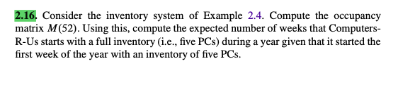
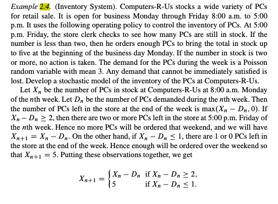
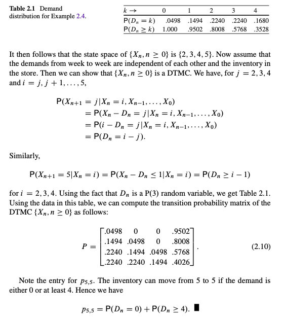
2.16. Consider the inventory system of Example 2.4. Compute the occupancy matrix M(52). Using this, compute the expected number of weeks that Computers- R-Us starts with a full inventory (i.e., five PCs) during a year given that it started the first week of the year with an inventory of five PCs. Example 2.4. (Inventory System). Computers-R-Us stocks a wide variety of PCs for retail sale. It is open for business Monday through Friday 8:00 a.m. to 5:00 p.m. It uses the following operating policy to control the inventory of PCs. At 5:00 p.m. Friday, the store clerk checks to see how many PCs are still in stock. If the number is less than two, then he orders enough PCs to bring the total in stock up to five at the beginning of the business day Monday. If the number in stock is two or more, no action is taken. The demand for the PCs during the week is a Poisson random variable with mean 3. Any demand that cannot be immediately satisfied is lost. Develop a stochastic model of the inventory of the PCs at Computers-R-Us. Let X,, be the number of PCs in stock at Computers-R-Us at 8:00 a.m. Monday of the nth week. Let D, be the number of PCs demanded during the nth week. Then the number of PCs left in the store at the end of the week is max(Xn - Dn, 0). If Xn- Dn 2, then there are two or more PCs left in the store at 5:00 p.m. Friday of the nth week. Hence no more PCs will be ordered that weekend, and we will have Xn+1 = X - Dn. On the other hand, if X - D 1, there are 1 or 0 PCs left in the store at the end of the week. Hence enough will be ordered over the weekend so that Xn+1 = 5. Putting these observations together, we get Xn+1 = { (Xn-Dn if Xn-Dn 2, if Xn - Dn 1. Table 2.1 Demand k-> 0 1 2 3 4 distribution for Example 2.4. P(Dn = k) P(Dn k) .0498 .1494 .2240 .2240 .1680 1.000 .9502 .8008 .5768 .3528 It then follows that the state space of {Xn, n 0} is {2, 3, 4, 5}. Now assume that the demands from week to week are independent of each other and the inventory in the store. Then we can show that {Xn, n > 0} is a DTMC. We have, for j = 2,3,4 and i = j, j + 1, ..., 5, P(Xn+1 = j|Xn = i, Xn-1,..., Xo) = P(Xn Dn = j|Xn =i, Xn1, ..., Xo) - = P(i Dn = j |X = i, Xn-1,..., Xo) - = P(Dn = i - j). Similarly, P(Xn+1=5|Xn = i) = P(Xn Dn 1|Xn = i) = P(Dn i 1) - for i = 2,3,4. Using the fact that D, is a P(3) random variable, we get Table 2.1. Using the data in this table, we can compute the transition probability matrix of the DTMC {Xn, n 0} as follows: .0498 0 0 .9502 .1494 .0498 0 .8008 P = .2240 .1494 .0498 .5768 L.2240 2240 .1494 .4026_ (2.10) Note the entry for p5,5. The inventory can move from 5 to 5 if the demand is either 0 or at least 4. Hence we have P5,5 = P(D=0) + P(Dn 4).